Google Code Jam Archive — Farewell Round D problems
Overview
Gardel used to sing in the famous "Volver" tango song that 20 years is nothing. It certainly does not feel that way for Coding Competitions. With these farewell rounds, a marvelous maze reaches the exit. Hopefully it was as entertaining and educational for you to solve it as it was for us to put it together.
For today's rounds we went with a Code Jam-finals setup for everyone: 4 hours, 5 problems, lots of problems with the same score. In this way, each contestant can trace their own path, as you have done throughout our history before.
Round A had all problems at newcomer level with all test sets visible, to align with a Coding Practice With Kick Start round. Round B was also fully visible, but had increasingly harder problems and required some techniques, like a Kick Start round. Rounds C and D had hidden test sets, ad-hoc ideas, some more advanced algorithms and data structures, and included an interactive problem, to cover the full spectrum of the Coding Competitions experience.
We also had appearances from Cody-Jamal, pancakes, names of famous computer scientists, a multi-part problem, I/O problem names, faux references to computer-world terms, and quite a few throwbacks to old problems.
Problems from these rounds will be up for practice until June 1st so you can get a chance at all of them before sign-in is disabled on the site.
Thanks to those of you who could join us today, and to everyone who was around in our long history. It has been amazing. Last words are always hard, so we can borrow from Gardel the ending of "Volver" that does fit the moment: "I save hidden a humble hope, which is all the fortune of my heart."
8
6245
876543
374300
350000
378385
21342
46727
112358
1
2
NA D
1
2 6
*Oo*.d
*cNCE*
Cast
Colliding Encoding: Written by Shashwat Badoni. Prepared by Jared Gillespie and Pablo Heiber.
Rainbow Sort: Written by Dmitry Brizhinev. Prepared by Shubham Avasthi.
Illumination Optimization: Written by Melisa Halsband. Prepared by Shaohui Qian.
Untie: Written and prepared by Pablo Heiber.
ASCII Art: Written by Bartosz Kostka. Prepared by Anveshi Shukla.
Collecting Pancakes: Written by Anurag Singh. Prepared by Pranav Gavvaji.
Spacious Sets: Written by Bartosz Kostka. Prepared by Deepanshu Aggarwal.
Intruder Outsmarting: Written by Muskan Garg. Prepared by Pablo Heiber and Saki Okubo.
Railroad Maintenance: Written by Emerson Lucena. Prepared by Mahmoud Ezzat.
Railroad Management: Written by Bintao Sun. Prepared by Yu-Che Cheng.
Game Sort: Part 1: Written by Luis Santiago Re and Pablo Heiber. Prepared by Isaac Arvestad and Luis Santiago Re.
Immunization Operation: Written by Chu-ling Ko. Prepared by Shaohui Qian.
Evolutionary Algorithms: Written by Anurag Singh. Prepared by Vinay Khilwani.
The Decades of Coding Competitions: Written by Ashish Gupta. Prepared by Bakuri Tsutskhashvili.
Game Sort: Part 2: Written by Luis Santiago Re. Prepared by Agustín Gutiérrez and Luis Santiago Re.
Indispensable Overpass: Written by Hsin-Yi Wang. Prepared by Shaohui Qian.
Ring-Preserving Networks: Written by Han-sheng Liu. Prepared by Pablo Heiber.
Hey Google, Drive!: Written by Archie Pusaka. Prepared by Chun-nien Chan.
Old Gold: Written and prepared by Ikumi Hide.
Genetic Sequences: Written and prepared by Max Ward.
Solutions and other problem preparation and review by Abhay Pratap Singh, Abhilash Tayade, Abhishek Saini, Aditya Mishra, Advitiya Brijesh, Agustín Gutiérrez, Akshay Mohan, Alan Lou, Alekh Gupta, Alice Kim, Alicja Kluczek, Alikhan Okas, Aman Singh, Andrey Kuznetsov, Anthony, Antonio Mendez, Anuj Asher, Anveshi Shukla, Arghya Pal, Arjun Sanjeev, Arooshi Verma, Artem Iglikov, Ashutosh Bang, Bakuri Tsutskhashvili, Balganym Tulebayeva, Bartosz Kostka, Chu-ling Ko, Chun-nien Chan, Cristhian Bonilha, Deeksha Kaurav, Deepanshu Aggarwal, Dennis Kormalev, Diksha Saxena, Dragos-Paul Vecerdea, Ekanshi Agrawal, Emerson Lucena, Erick Wong, Gagan Kumar, Han-sheng Liu, Harshada Kumbhare, Harshit Agarwala, Hsin-Yi Wang, Ikumi Hide, Indrajit Sinha, Isaac Arvestad, Jared Gillespie, Jasmine Yan, Jayant Sharma, Ji-Gui Zhang, Jin Gyu Lee, John Dethridge, João Medeiros, Junyang Jiang, Katharine Daly, Kevin Tran, Kuilin Wang, Kushagra Srivastava, Lauren Minchin, Lucas Maciel, Luis Santiago Re, Marina Vasilenko, Mary Yang, Max Ward, Mayank Aharwar, Md Mahbubul Hasan, Mo Luo, Mohamed Yosri Ahmed, Mohammad Abu-Amara, Murilo de Lima, Muskan Garg, Nafis Sadique, Nitish Rai, Nurdaulet Akhanov, Olya Kalitova, Ophelia Doan, Osama Fathy, Pablo Heiber, Pawel Zuczek, Raghul Rajasekar, Rahul Goswami, Raymond Kang, Ritesh Kumar, Rohan Garg, Ruiqing Xiang, Sadia Atique, Sakshi Mittal, Salik Mohammad, Samiksha Gupta, Samriddhi Srivastava, Sanyam Garg, Sara Biavaschi, Sarah Young, Sasha Fedorova, Shadman Protik, Shantam Agarwal, Sharmin Mahzabin, Sharvari Gaikwad, Shashwat Badoni, Shu Wang, Shubham Garg, Surya Upadrasta, Swapnil Gupta, Swapnil Mahajan, Tanveer Muttaqueen, Tarun Khullar, Thomas Tan, Timothy Buzzelli, Tushar Jape, Udbhav Chugh, Ulises Mendez Martinez, Umang Goel, Viktoriia Kovalova, Vinay Khilwani, Vishal Som, William Di Luigi, Yang Xiao, Yang Zheng, Yu-Che Cheng, and Zongxin Wu.
Analysis authors:
- Colliding Encoding: Surya Upadrasta.
- Rainbow Sort: Rakesh Theegala.
- Illumination Optimization: Sarah Young.
- Untie: Pablo Heiber.
- ASCII Art: Raghul Rajasekar.
- Collecting Pancakes: Raghul Rajasekar.
- Spacious Sets: Rakesh Theegala.
- Intruder Outsmarting: Ekanshi Agrawal.
- Railroad Maintenance: Cristhian Bonilha.
- Railroad Management: Emerson Lucena.
- Game Sort: Part 1: Mohamed Yosri Ahmed.
- Immunization Operation: Sadia Atique.
- Evolutionary Algorithms: Krists Boitmanis.
- The Decades of Coding Competitions: Chun-nien Chan.
- Game Sort: Part 2: Agustín Gutiérrez.
- Indispensable Overpass: Arooshi Verma.
- Ring-Preserving Networks: Han-sheng Liu.
- Hey Google, Drive!: Chu-ling Ko.
- Old Gold: Evan Dorundo.
- Genetic Sequences: Max Ward.
A. Indispensable Overpass
Problem
A modern railroad system built in Ekiya's town bumped into a major hurdle: the main freeway running north to south. $$$\mathbf{W}$$$ stations have already been built and connected on the western side of the freeway and $$$\mathbf{E}$$$ on the eastern side. One more connection is needed between a western and an eastern station, but because the freeway is in the way, that connection needs to be built using an overpass.
Ekiya is assessing which stations would be most convenient to connect with the overpass. As part of that assessment, she wants to know how the average length (in number of stations) of a path within the system might change with each possible option.
A path between stations $$$s$$$ and $$$t$$$ is a list of distinct stations that starts with $$$s$$$, ends with $$$t$$$, and such that any two consecutive stations on the list share a connection. The railroad system currently has $$$\mathbf{W}$$$ stations on the western side, connected through $$$\mathbf{W}-1$$$ connections such that there is exactly one path between any two distinct western stations. Similarly, there are $$$\mathbf{E}$$$ eastern stations connected through $$$\mathbf{E}-1$$$ connections such that there is exactly one path between any two distinct eastern stations. After the overpass connection is built connecting one western and one eastern station, there will be exactly one path between any two distinct stations.
A complete map is a map that has $$$\mathbf{W}+\mathbf{E}-1$$$ total connections and exactly one path between any pair of stations. The average distance of a complete map is the average of the length of paths between all pairs of different stations. The length of a path is one less than the length of the list of stations that defines it (e.g., the path between directly connected stations has a length of $$$1$$$).
As an example, the picture below illustrates a scenario with $$$\mathbf{W} = 2$$$ stations on the west side and $$$\mathbf{E} = 3$$$ stations on the east side. There are $$$2$$$ possible overpasses shown.
This table shows the lengths of the paths between pairs of stations if each overpass were to be built.
| $$$\color{darkred}{\mathbf{1 \leftrightarrow 1}}$$$ | $$$\color{darkblue}{\mathbf{2 \leftrightarrow 3}}$$$ | ||
|---|---|---|---|
| West $$$1$$$ | West $$$2$$$ | $$$1$$$ | $$$1$$$ |
| West $$$1$$$ | East $$$1$$$ | $$$1$$$ | $$$3$$$ |
| West $$$1$$$ | East $$$2$$$ | $$$3$$$ | $$$3$$$ |
| West $$$1$$$ | East $$$3$$$ | $$$2$$$ | $$$2$$$ |
| West $$$2$$$ | East $$$1$$$ | $$$2$$$ | $$$2$$$ |
| West $$$2$$$ | East $$$2$$$ | $$$4$$$ | $$$2$$$ |
| West $$$2$$$ | East $$$3$$$ | $$$3$$$ | $$$1$$$ |
| East $$$1$$$ | East $$$2$$$ | $$$2$$$ | $$$2$$$ |
| East $$$1$$$ | East $$$3$$$ | $$$1$$$ | $$$1$$$ |
| East $$$2$$$ | East $$$3$$$ | $$$1$$$ | $$$1$$$ |
| Average: | $$$2$$$ | $$$1.8$$$ |
Given the current stations and connections, and a list of options for the overpass connection, help Ekiya by calculating the average distance of the map that would result if that option was the only overpass connection built.
Input
The first line of the input gives the number of test cases, $$$\mathbf{T}$$$. $$$\mathbf{T}$$$ test cases follow. Each test case starts with a line with three integers $$$\mathbf{W}$$$, $$$\mathbf{E}$$$, and $$$\mathbf{C}$$$, the number of western and eastern stations, and the number of options for the overpass connection, respectively. Western stations are numbered between $$$1$$$ and $$$\mathbf{W}$$$ and eastern connections are numbered between $$$1$$$ and $$$\mathbf{E}$$$.
The second line of a test case contains $$$\mathbf{W}-1$$$ integers $$$\mathbf{X_1}, \mathbf{X_2}, \dots, \mathbf{X_{W-1}}$$$ representing that the $$$i$$$-th existing connection among western stations connects western stations $$$i$$$ and $$$\mathbf{X_i}$$$.
The third line of a test case contains $$$\mathbf{E}-1$$$ integers $$$\mathbf{F_1}, \mathbf{F_2}, \dots, \mathbf{F_{E-1}}$$$ representing that the $$$j$$$-th existing connection among eastern stations connects eastern stations $$$j$$$ and $$$\mathbf{F_j}$$$.
Finally, the last $$$\mathbf{C}$$$ lines of a test case describe the options for the overpass connection. The $$$k$$$-th of these lines contains two integers $$$\mathbf{A_k}$$$ and $$$\mathbf{B_k}$$$ representing the western and eastern stations, respectively, that the $$$k$$$-th option for an overpass connection would connect.
Output
For each test case, output one line containing
Case #$$$x$$$: $$$y_1 ~ y_2 ~ \cdots ~ y_{\mathbf{C}}$$$,
where $$$x$$$ is the test case number (starting from 1) and $$$y_k$$$ is the average distance of
the map resulting in adding the $$$k$$$-th option as an overpass connection to all existing
connections.
$$$y_1$$$, $$$y_2$$$, $$$\dots$$$ and $$$y_k$$$ will be considered correct if they are within an
absolute or relative error of $$$10^{-6}$$$ of the correct answer. See the
FAQ
for an explanation of what that means, and what formats of real numbers
we accept.
Limits
Memory limit: 2 GB.
$$$1 \le \mathbf{T} \le 100$$$.
$$$2 \le \mathbf{W} \le 10^5$$$.
$$$2 \le \mathbf{E} \le 10^5$$$.
$$$i + 1 \le \mathbf{X_i} \le \mathbf{W}$$$, for all $$$i$$$.
(This implies that there is exactly one path between each pair of western stations.)
$$$j + 1 \le \mathbf{F_j} \le \mathbf{E}$$$, for all $$$j$$$.
(This implies that there is exactly one path between each pair of eastern stations.)
$$$1 \le \mathbf{A_k} \le \mathbf{W}$$$, for all $$$k$$$.
$$$1 \le \mathbf{B_k} \le \mathbf{E}$$$, for all $$$k$$$.
$$$(\mathbf{A_k}, \mathbf{B_k}) \neq (\mathbf{A_\ell}, \mathbf{B_\ell})$$$, for all $$$k \neq \ell$$$. (Each listed overpass
connection is different.)
Test Set 1 (Visible Verdict)
Time limit: 20 seconds.
$$$1 \le \mathbf{C} \le 2$$$.
Test Set 2 (Hidden Verdict)
Time limit: 40 seconds.
$$$1 \le \mathbf{C} \le 10^5$$$.
Sample
3
2 3 2
2
3 3
1 1
2 3
3 4 2
2 3
3 3 4
1 3
1 2
3 4 1
2 3
3 3 4
2 2
Case #1: 2.0 1.8
Case #2: 2.19047619 2.47619048
Case #3: 2.2857142857
Sample Case #1 is explained and illustrated in the problem statement. Sample Case #2 and Sample Case #3 are illustrated below.
B. Genetic Sequences
Genetic Sequences
Margaret researches genetic sequences. She is analysing two sequences $$$\mathbf{A}$$$ and $$$\mathbf{B}$$$ from a new kind
of life that does not use the typical four letter genetic alphabet.
The code for the genetic sequences conveniently requires $$$26$$$ letters represented by the
uppercase English letters 'A' through 'Z'.
Margaret wants to compare the sequences $$$\mathbf{A}$$$ and $$$\mathbf{B}$$$. The best way to do this is to do a series of sequence analysis tests. Each test involves taking a prefix from $$$\mathbf{A}$$$ containing only the first $$$\mathbf{P}$$$ letters from $$$\mathbf{A}$$$, which is called the $$$\mathbf{A}$$$-prefix. Each test also involes taking a suffix from $$$\mathbf{B}$$$ containing only the last $$$\mathbf{S}$$$ letters from $$$\mathbf{B}$$$, which is called the $$$\mathbf{B}$$$-suffix. Margaret then needs to compare the $$$\mathbf{A}$$$-prefix to the $$$\mathbf{B}$$$-suffix. A substring is a subsequence of contiguous letters. A substring from the $$$\mathbf{A}$$$-prefix matches the $$$\mathbf{B}$$$-suffix if the $$$\mathbf{B}$$$-suffix starts with that substring. That is, the substring is a prefix of the $$$\mathbf{B}$$$-suffix. The result of a test is the length of the longest substring from the $$$\mathbf{A}$$$-prefix that matches the $$$\mathbf{B}$$$-suffix.
Margaret needs some software to determine the outcome of a batch of $$$\mathbf{Q}$$$ sequence analysis tests. Note that each test is independent. Margaret has many copies of $$$\mathbf{A}$$$ and $$$\mathbf{B}$$$ and a new one is used for each test.
Input
The first line of the input gives the number of test cases, $$$\mathbf{T}$$$. $$$\mathbf{T}$$$ test cases follow. Each test case begins with a line containing two strings and an integer, $$$\mathbf{A}$$$, $$$\mathbf{B}$$$, and $$$\mathbf{Q}$$$ respectively. Each test case ends with $$$\mathbf{Q}$$$ lines, the $$$i$$$-th of which contains two integers $$$\mathbf{P_i}$$$ and $$$\mathbf{S_i}$$$, which are the prefix and suffix sizes for the $$$i$$$-th sequence analysis test.
Output
For each test case, output one line containing
Case #$$$x$$$: $$$y_1 ~ y_2 ~ \dots ~ y_{\mathbf{Q}}$$$,
where $$$x$$$ is the test case number (starting from 1) and $$$y_i$$$ is the answer to the
$$$i$$$-th query in the input.
Limits
Time limit: 20 seconds.
Memory limit: 2 GB.
$$$1 \le \mathbf{T} \le 100$$$.
$$$1 \leq \mathbf{P_i} \leq $$$ the length of $$$\mathbf{A}$$$.
$$$1 \leq \mathbf{S_i} \leq $$$ the length of $$$\mathbf{B}$$$.
Test Set 1 (Visible Verdict)
$$$1 \le $$$ the length of $$$ \mathbf{A} \le 3000$$$.
$$$1 \le $$$ the length of $$$ \mathbf{B} \le 3000$$$.
$$$1 \le \mathbf{Q} \le 3000$$$.
Test Set 2 (Hidden Verdict)
$$$1 \le $$$ the length of $$$ \mathbf{A} \le 10^5$$$.
$$$1 \le $$$ the length of $$$ \mathbf{B} \le 10^5$$$.
The sum of the lengths of $$$\mathbf{A}$$$ over all test cases is $$$\leq 5 \times 10^5$$$
The sum of the lengths of $$$\mathbf{B}$$$ over all test cases is $$$\leq 5 \times 10^5$$$
$$$1 \le \mathbf{Q} \le 10^5$$$.
Sample
3
ABCABAC CABABA 3
3 6
7 6
6 5
BANANA HABANA 2
5 4
5 5
ABC ABD 1
2 1
Case #1: 1 4 3
Case #2: 4 1
Case #3: 0
In Sample Case #1, there are 3 tests. The prefix ABC from $$$\mathbf{A}$$$ and the complete suffix
CABABA from $$$\mathbf{B}$$$ are compared in the first test. The answer is 1, since C
is the longest substring that is contained in ABC and is a prefix of
CABABA. In the second test, ABCABAC is tested against
CABABA and the longest match is CABA. In the third test, ABCABA
is tested against ABABA and the longest match is ABA.
In Sample Case #2, there are 2 tests. In the first, BANAN is tested against
BANA, and the longest match is BANA. In the second, BANAN
is tested against ABANA, and the longest match is A.
In Sample Case #3, there is one test. In it, AB is tested against D.
Since there is no match the answer is 0.
C. Hey Google, Drive!
Problem
The Google Assistant and Android Auto teams are collaborating on a new prototype car that can be driven via voice commands. The early prototype works through a phone connected to a car simulator. Unfortunately, one of the early testers dropped their phone in the toilet, damaging the microphone and making it harder to use the new feature. Since they do not want to miss out on the opportunity, they want your help to use it anyway.
The early prototype moves on a simple grid of $$$\mathbf{R}$$$ rows and $$$\mathbf{C}$$$ columns and only understands $$$4$$$ very simple voice commands: north, south, east, and west. Each command makes the car try to move exactly one cell in the corresponding direction. Because of the microphone issues, however, the system may mishear and interchange north and south, and separately, east and west. That means that a command of north may make the car move north or south, a command of south may make the car move south or north, and similarly both commands east and west may make the car move east or west when issued. In all cases, both movement options can happen with equal probability ($$$1/2$$$).
The tester set up a driving grid such that each cell can contain either a wall, a hazard, or be empty. If a command would make the car move into a wall, or outside the grid, it does nothing instead. If a command makes the car move into a hazard, the car cannot execute any more commands.
The tester has marked some empty cells of the grid as interesting starts and others as interesting finishes. A pair of an interesting start and an interesting finish is drivable if there is a strategy to drive the car through voice commands from the start that makes it end at the finish with probability at least $$$1 - 10^{-{10^{100}}}$$$. A strategy can choose which command to issue and when to stop depending on the outcome of the previous commands. Notice that if the car moves into a hazard it stops moving, so it cannot make it to the finish. The tester wants your help finding the list of all drivable pairs.
Input
The first line of the input gives the number of test cases, $$$\mathbf{T}$$$. $$$\mathbf{T}$$$ test cases follow. Each test case starts with a line containing two integers $$$\mathbf{R}$$$ and $$$\mathbf{C}$$$, the number of rows and columns of the grid. Then, $$$\mathbf{R}$$$ lines follow containing a string of $$$\mathbf{C}$$$ characters each. The $$$j$$$-th character on the $$$i$$$-th of these lines $$$\mathbf{G_{i,j}}$$$ represents the grid in the $$$i$$$-th row and $$$j$$$-th column as follows:
- A period (
.) represents an uninteresting empty cell. - A hash symbol (
#) represents a cell containing a wall. - An asterisk (
*) represents a cell containing a hazard. - An English lowercase letter (
athroughz) represents an empty cell that is an interesting start. - An English uppercase letter (
AthroughZ) represents an empty cell that is an interesting finish.
Output
For each test case, output one line containing
Case #$$$x$$$: $$$y$$$,
where $$$x$$$ is the test case number (starting from 1) and $$$y$$$ is NONE if there
are no drivable pairs. Otherwise, $$$y$$$ must be a series of $$$2$$$ character strings separated
by spaces, representing all drivable pairs with the start letter first and the finish letter
second, in alphabetical order.
Limits
Time limit: 60 seconds.
Memory limit: 2 GB.
$$$1 \le \mathbf{T} \le 100$$$.
$$$\mathbf{G_{i,j}}$$$ is either a period (.), a hash symbol (#), an asterisk
(*) or a lowercase or uppercase English letter, for all $$$i, j$$$.
The set $$$\{\mathbf{G_{i,j}}$$$ for all $$$i, j\}$$$ contains at least $$$1$$$ lowercase
and at least $$$1$$$ uppercase English letter.
Each lowercase and uppercase letter appears at most once among all $$$\mathbf{G_{i,j}}$$$.
Test Set 1 (Visible Verdict)
$$$1 \le \mathbf{R} \le 20$$$.
$$$1 \le \mathbf{C} \le 20$$$.
Test Set 2 (Hidden Verdict)
$$$1 \le \mathbf{R} \le 100$$$.
$$$1 \le \mathbf{C} \le 100$$$.
Sample
4
1 2
aZ
4 4
a..c
**.*
.Y.#
bX#Z
2 2
a*
*Z
2 7
a*bcd*.
...*F#.
Case #1: aZ
Case #2: aY bX bY cY
Case #3: NONE
Case #4: dF
In Sample Case #1, simply repeating the west command until reaching the finish is a viable strategy. Each time there is a $$$1/2$$$ probability of reaching the finish and a $$$1/2$$$ probability of staying in the same place. Thus, the probability of not reaching the finish in $$$10^{101}$$$ or fewer steps is $$$2^{-10^{101}} \lt 10^{-10^{100}}$$$.
In Sample Case #2 a similar strategy as in Sample Case #1 can be used to get the car
from any position in the top row (1) to any other with probability as high as desired,
and similarly for all non-wall positions in the third row from the top (2). Analogously,
but using the south command, the car can move between non-wall positions on the third column
from the left (3).
From both a and c we can use (1) to get to the third column from the
left, then (3) to get right next to Y and then (2) to get to Y making
both aY and cY drivable. Notice, however, that safely using the north
or south commands from the third row can only be done in the third column, or otherwise the car
may go into a hazard. Therefore, there is no safe way to move the car from the third to the
fourth row, making aX and cX not drivable.
From b, however, the car can use a similar strategy to get to X, and
from X the car can get to Y by using the north or south command
repeatedly (and stop when reaching Y, never risking going into the hazard
above).
Finally, the finish Z is completely isolated, so it cannot be part of a drivable
pair.
In Sample Case #3, every path from the interesting start to the interesting finish goes through a hazard, which makes the pair not drivable.
In Sample Case #4, only the interesting start d has a viable strategy to get to the
finish F.
D. Old Gold
Problem
A long, long time ago ($$$7$$$ years) you were in a West-East road in southeast Asia known to contain at least one gold nugget, with a limited but reliable gold detector. After getting immensely rich with that gold, you have tried and got bored of every conceivable activity. While wandering around your huge mansion you found some notes from that gold hunt.
The notes are in the form of a diagram of the road. For each kilometer of road, you have one of $$$5$$$ markings:
<, indicating that the closest gold nugget is to the West,=, indicating that the closest gold nuggets to the East and to the West are at the same distance, and no gold nugget is at that position,>, indicating that the closest gold nugget is to the East,o, indicating that there is a gold nugget at that position, or., indicating that nothing is known about that location.
Since each of the $$$k$$$ unknown (.) positions could contain or not contain a gold
nugget independently, you want to find out how many of the $$$2^k$$$ placements of gold
are compatible with all your notes and result in the road overall containing at least one gold nugget. Since the output can be a really big number,
we only ask you to output the remainder of dividing the result by the prime
$$$10^9+7$$$ ($$$1000000007$$$).
Input
The first line of the input gives the number of test cases, $$$\mathbf{T}$$$. $$$\mathbf{T}$$$ lines follow. Each line contains a string $$$\mathbf{S}$$$ representing a single test case. The $$$i$$$-th character of $$$\mathbf{S}$$$ represents the marking in your notes for the $$$i$$$-th kilometer of road, from West to East, using the code explained above.
Output
For each test case, output one line containing Case #$$$x$$$: $$$y$$$,
where $$$x$$$ is the test case number (starting from 1) and $$$y$$$ is the number of
different gold placements that are compatible with your notes, modulo the prime
$$$10^9+7$$$ ($$$1000000007$$$).
Limits
Memory limit: 2 GB.
$$$1 \le \mathbf{T} \le 100$$$.
Each character of $$$\mathbf{S}$$$ is either < (less than), = (equals),
> (greater than), o (lowercase o), or . (period).
At least $$$1$$$ and not all characters of $$$\mathbf{S}$$$ are . (period).
Test Set 1 (Visible Verdict)
Time limit: 20 seconds.
$$$2 \le $$$ the length of $$$\mathbf{S} \le 100$$$.
Test Set 2 (Hidden Verdict)
Time limit: 40 seconds.
$$$2 \le $$$ the length of $$$\mathbf{S} \le 5 \times 10^5$$$.
Sample
4
o..=>..
...o>..........
.=.
.........o........
Case #1: 3
Case #2: 0
Case #3: 1
Case #4: 131072
In Sample Case #1, there are three valid placements resulting in roads oo<=>o<,
oo<=>oo and o<<=>>o.
In Sample Case #2, there is no valid placement.
In Sample Case #3, the only valid placement results in road o=o.
Note that a valid placement must always result in a road containing at least one gold nugget.
In Sample Case #4, all $$$2^{17}$$$ placements are valid. In this case,
a placement selecting to leave all the unknown (.) positions empty (without a gold nugget)
is valid because the road overall still has one gold nugget in such a placement.
E. Ring-Preserving Networks
Problem
A research consortium is building a new datacenter. In the datacenter, a set of computers is set up to work together and communicate via a network. The network works only with direct bidirectional links between computers. After the success of their name-preserving networks, they decided to do other designs with guaranteed properties.
The consortium has asked you to submit a design of a ring-preserving network. We define a ring of a network as an ordering of all the computers of the network such that any two computers that are consecutive in the ordering have a direct link between them, and the same is true for the first and last computers in the ordering.
A ring-preserving network is a network design that can efficiently find a ring of itself even after losing the original computer identifications. You need to submit several network designs that are ring-preserving.
To evaluate your network designs, the research consortium has set up an automated program. You will be asked for network designs specifying the exact number of computers $$$\mathbf{C}$$$ and the exact number of bidirectional links $$$\mathbf{L}$$$ it must contain. You must assign each computer a unique ID between $$$1$$$ and $$$\mathbf{C}$$$ and list the $$$\mathbf{L}$$$ links using the IDs to refer to the links' endpoints. The evaluating program will receive that design and send back a copy of the network design with the following changes:
- the unique IDs have been permuted uniformly at random (that is, each ID is now equally likely to be on any of the computers),
- every link is listed with the smallest ID first (using the new IDs), and
- the set of links is listed in increasing order of the first endpoint (using the new IDs), breaking ties by smallest second endpoint (i.e., lexicographical order).
You need to be able to find a ring of the modified network. It does not need to be the original ring.
Input and output
This is an interactive problem. You should make sure you have read the information in the Interactive Problems section of our FAQ.
Initially, your program should read a single line containing an integer, $$$\mathbf{T}$$$, the number of test cases. Then, $$$\mathbf{T}$$$ test cases must be processed.
For each test case, your program must first read a line containing two integers $$$\mathbf{C}$$$ and $$$\mathbf{L}$$$: the number of computers and links to include in the network design.
Then, you need to create a network design with $$$\mathbf{C}$$$ computers and $$$\mathbf{L}$$$ links and print exactly $$$\mathbf{L}$$$ lines representing that design. Each of these lines must contain two integers A and B each, representing a different link between computers A and B, where $$$A \ne B$$$. Notice that if you list link A B, you may not list A B nor B A again.
Upon reading your network design, the judge will send you $$$\mathbf{L}$$$ lines back representing the permuted design. The $$$i$$$-th of these lines contains two integers $$$\mathbf{U_i}$$$ and $$$\mathbf{V_i}$$$ representing a bidirectional link between the computers with new ids $$$\mathbf{U_i}$$$ and $$$\mathbf{V_i}$$$. The copy is generated using a permutation chosen uniformly at random from all possible permutations, and independently of any other choices.
To finish a test case, you need to send the judge a single line with $$$\mathbf{C}$$$ integers $$$x_1, x_2, \dots, x_\mathbf{C}$$$, representing a ring of the permuted design. That is, the set of lines the judge sent back must include either $$$x_1\ x_\mathbf{C}$$$ or $$$x_\mathbf{C}\ x_1$$$, and, for all $$$i$$$, it must include either $$$x_i\ x_{i+1}$$$ or $$$x_{i+1}\ x_i$$$.
You should not send additional information to the judge after solving all test cases. In other words, if your program keeps printing to standard output after printing the list of $$$x$$$s for the last test case, you will receive a Wrong Answer judgment.
If at any point the judge reads from your program malformed input (wrong number of tokens, non-integer tokens or out of range numbers) it will immediately stop and assume Wrong Answer. However, if your program happens to remain waiting for input from the judge, it may end up exceeding the time limit and receiving a Time Limit Exceeded judgement. On the other hand, if you commit a recoverable error (sending over a network with a repeated connection, or a connection from a computer to itself, or sending a ring that repeats a computer or that uses an edge that does not exist in the permuted version) the judge will continue to communicate with your program trying to finish, but the overall judgement will be Wrong Answer.
Notice that you are allowed to submit the same network design for different test cases, as long as that design complies with all restrictions for both cases. Additionally, the seed for random generation in the judge is fixed, so sending the same set of original network designs in the same order will get back the same set of copies.
Limits
Time limit: 30 seconds.
Memory limit: 2 GB.
$$$1 \le \mathbf{T} \le 100$$$.
$$$3 \le \mathbf{C} \le 10000$$$.
$$$\mathbf{C} \le \mathbf{L} \le \mathbf{C} \times (\mathbf{C} - 1) / 2$$$.
$$$1 \le \mathbf{U_i} \lt \mathbf{V_i} \le \mathbf{C}$$$, for all $$$i$$$.
$$$\mathbf{U_i} \le \mathbf{U_{i+1}}$$$, for all $$$i$$$.
If $$$\mathbf{U_i} = \mathbf{U_{i+1}}$$$ then $$$\mathbf{V_i} \le \mathbf{V_{i+1}}$$$, for all $$$i$$$.
There exist permutations $$$f$$$ of length $$$\mathbf{C}$$$ and $$$g$$$ of length $$$\mathbf{L}$$$ such that, for each $$$i$$$,
if $$$A\ B$$$ is the $$$g(i)$$$-th line in your original design, then
$$$\{\mathbf{U_i}, \mathbf{V_i}\} = \{f(A), f(B)\}$$$. (The given links result from applying a permutation
of computer IDs to the ones you gave, and then sorting the links lexicographically).
Test Set 1 (Visible Verdict)
$$$\mathbf{L} \le \mathbf{C} + 10$$$.
Test Set 2 (Hidden Verdict)
$$$\mathbf{L} \le 20000$$$.
Testing Tool
You can use this testing tool to test locally or on our platform. To test locally, you will need to run the tool in parallel with your code; you can use our interactive runner for that. For more information, read the instructions in comments in that file, and also check out the Interactive Problems section of the FAQ.
Instructions for the testing tool are included in comments within the tool. We encourage you to add your own test cases. Please be advised that although the testing tool is intended to simulate the judging system, it is NOT the real judging system and might behave differently. If your code passes the testing tool but fails the real judge, please check the Coding section of the FAQ to make sure that you are using the same compiler as us.
2
4 5
1 2
1 3
4 2
4 3
1 4
1 2
1 3
1 4
2 4
3 4
1 2 4 2
4 4
1 2
1 4
3 2
3 4
1 2
1 3
2 4
3 4
2 1 3 4
Analysis — A. Indispensable Overpass
Test Set 1
A brute-force solution would be to calculate and sum the distances between every pair of stations, then divide by the total number of pairs. The total number of stations is $$$\mathbf{W} + \mathbf{E}$$$, which means that there are $$$N = \frac{(\mathbf{W} + \mathbf{E}) \times (\mathbf{W} + \mathbf{E} - 1)}{2}$$$ total pairs of stations. Calculating the distance between any given pair takes $$$O(\mathbf{W} + \mathbf{E})$$$ time, so this solution has a time complexity of $$$O((\mathbf{W} + \mathbf{E})^3)$$$, which is too slow.
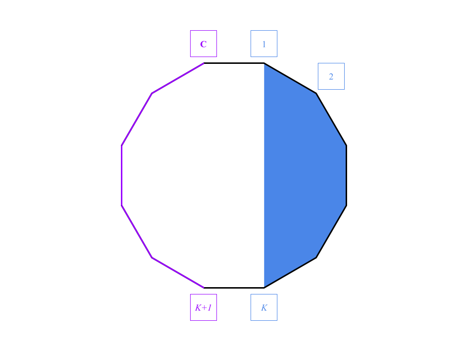
First notice that the western stations make a tree, because there is exactly one path between any two stations. This also applies to the eastern stations. Let us define the western tree as $$$T_W$$$, the eastern tree as $$$T_E$$$, and the tree created by connecting the two trees as $$$T_{W+E}$$$.
Instead of calculating the distances between every pair of stations, we can instead compute how many paths go through each edge, which we call the "contribution" of each edge, in $$$T_{W+E}$$$. The total sum of all distances between pairs of nodes is equal to the total sum of edge contributions. We just have to sum up these contributions and divide by $$$N$$$ to get the average distance for the given case.
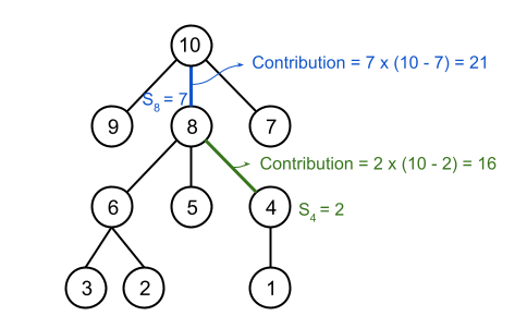
To compute an edge's contribution, we need two depth-first-search (DFS) traversals. First, choose an arbitrary root $$$r$$$ in $$$T_{W+E}$$$. For the first traversal, for each node $$$n$$$ starting from $$$r$$$, compute and store the size of the subtree $$$S_n$$$ under $$$n$$$. This can be calculated recursively by $$$S_n = 1 + \sum_i S_i$$$, where the sum is over all children $$$i$$$ of $$$n$$$. Fig.1 has an example shown below.
.png)
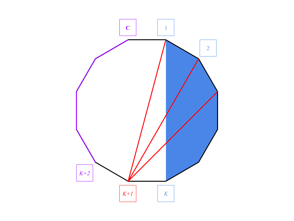
Then, traverse the tree a second time to compute each edge's contribution. The key insight here is that for an edge between nodes $$$n$$$ and $$$p$$$, where $$$n$$$ is the child of $$$p$$$, the edge's contribution is equal to $$$S_n \times (\mathbf{W} + \mathbf{E} - S_n)$$$. Thus, the second traversal goes through all the edges in $$$T_{W+E}$$$ and calculates their contributions using the stored subtree sizes from the first traversal. This is demonstrated below in Fig.2.
Afterwards, summing up the edge contributions and dividing by $$$N$$$ yields the answer. Since the two traversals take $$$O(\mathbf{W} + \mathbf{E})$$$ each, and we need to redo the traversals for each of the $$$\mathbf{C}$$$ cases, the total time complexity is $$$O((\mathbf{W} + \mathbf{E}) \times \mathbf{C})$$$. This is sufficient for Test Set 1, but not for Test Set 2.
Test Set 2
The key insight for Test Set 2 is that the total path sum of the $$$N$$$ pairs can be computed from the formula $$$\mathbf{E} \times P^W_{\mathbf{A_k}} + \mathbf{W} \times P^E_{\mathbf{B_k}} + \mathbf{W} \times \mathbf{E} + Q^W + Q^E$$$, where $$$P^W_n$$$ is the path sum from node $$$n$$$ to all other nodes in $$$T_W$$$, $$$Q^W$$$ is the total path sum within $$$T_W$$$, and likewise for $$$P^E_n$$$ and $$$Q^E$$$. If these values are precomputed already, then whenever we are given a connection $$$(\mathbf{A_k}, \mathbf{B_k})$$$, we can return the average distance in a constant time operation using the formula above. Before deriving this formula, let us first find out how to precompute $$$Q^W, Q^E$$$, and $$$P^W_n, P^E_n$$$ for each node $$$n$$$ efficiently first. This can be accomplished with two DFS traversals for both $$$T_W$$$ and $$$T_E$$$ individually.
Let us look at $$$T_W$$$ for convenience. For the first DFS, starting from an arbitrary root $$$r$$$, calculate at each node $$$n$$$:
- The size of the subtree rooted by $$$n$$$, defined as $$$S^W_n$$$. This can be calculated recursively by $$$S^W_n = 1 + \sum_i S^W_i$$$, where the sum is over all children $$$i$$$ of $$$n$$$.
- The path sum from $$$n$$$ to all its descendants, defined as $$$D^W_n$$$. This can be computed recursively by $$$D^W_n = \sum_{i} D^W_i + (S_n-1)$$$, where the sum is over all children $$$i$$$ of $$$n$$$.
.png)
This first traversal calculates the number of subtrees and subtree path sums below $$$n$$$. However, $$$D^W_n$$$ is not the full sum of all paths from $$$n$$$ to other nodes in $$$T_W$$$ because we only counted paths travelling downwards from $$$n$$$. For every node, we also need to compute path sums that go above and through its parent. This is done via a second DFS. In this traversal, given a node $$$n$$$ and its parent $$$p$$$, the actual path sum $$$P^W_n$$$ is computed as follows:
$$$P^W_n = D^W_n + (\mathbf{W} - S^W_n) + (P^W_p - (D^W_n + S^W_n))$$$
Essentially, we add onto $$$D^W_n$$$ two values:
- $$$(\mathbf{W} - S^W_n)$$$, the contribution of the edge connecting $$$n$$$ to $$$p$$$
- $$$P^W_p - (D^W_n + S^W_n)$$$, the path sums starting from $$$p$$$ that do not go through $$$n$$$.
For the root $$$r$$$ of $$$T_W$$$, $$$P^W_r = D^W_r$$$, as shown below in Fig.4.
+(Pp-Dn-Sn).png)
With $$$P^W_n$$$ computed for all nodes $$$n$$$ in $$$T_W$$$ and again $$$P^E_n$$$ computed for all nodes in $$$T_E$$$, we can calculate the average distance for each case in constant time. Now let us derive the formula mentioned earlier. Suppose we are given a connection between $$$\mathbf{A_k}$$$ from the west, and $$$\mathbf{B_k}$$$from the east. We first note that the total path sum can be computed as:
$$$\sum_{i \in T_W} \sum_{j \in T_E} d_{i,j} + Q^W + Q^E$$$
where $$$d_{i,j}$$$ is the distance between nodes $$$i$$$ and $$$j$$$. Here, $$$Q^W$$$ is the sum of all paths in $$$T_W$$$, and $$$Q^E$$$ is the sum of all paths in $$$T_E$$$. We can already calculate them just by summing the $$$P_n$$$s on each side.
$$$Q^W = \frac{\sum_{n \in T_W} P^W_n}{2}, Q^E = \frac{\sum_{n \in T_E} P^E_n}{2}$$$
The first sum about $$$d_{i,j}$$$ is trickier, but we can separate it into three terms that incorporate $$$\mathbf{A_k}$$$ and $$$\mathbf{B_k}$$$:
$$$\sum_{i \in T_W} \sum_{j \in T_E} (d_{i,\mathbf{A_k}} + d_{j,\mathbf{B_k}} + 1)$$$.
All the terms now allow us to simplify the double summation to single summations. The above equation is equivalent to:
$$$\mathbf{E} \times \sum_{i \in T_W} d_{i,\mathbf{A_k}} + \mathbf{W} \times \sum_{j \in T_E} d_{j,\mathbf{B_k}} + \mathbf{W} \times \mathbf{E}$$$.
Because we precomputed all the path sums, $$$\sum_{i \in T_W} d_{i,\mathbf{A_k}}$$$ is equal to $$$P^W_{\mathbf{A_k}}$$$, and $$$\sum_{j \in T_E} d_{j,\mathbf{B_k}}$$$ is equal to $$$P^E_{\mathbf{B_k}}$$$. Thus, the total path distances between the two trees is
$$$\mathbf{E} \times P^W_{\mathbf{A_k}} + \mathbf{W} \times P^E_{\mathbf{B_k}} + \mathbf{W} \times \mathbf{E} + Q^W + Q^E$$$.
Divide that by $$$N$$$ to get the average distance for each query. Each traversal for $$$T_W$$$ and $$$T_E$$$ is $$$O(\mathbf{W})$$$ and $$$O(\mathbf{E})$$$ respectively, which makes the overall complexity $$$O(\mathbf{W} + \mathbf{E} + \mathbf{C})$$$ for $$$\mathbf{C}$$$ cases.
Analysis — B. Genetic Sequences
Test Set 1
The problem asks us to answer queries on two strings $$$\mathbf{A}$$$ and $$$\mathbf{B}$$$. In each query, we are given an $$$\mathbf{A}$$$-prefix and a $$$\mathbf{B}$$$-suffix. We are asked to find the longest prefix of the $$$\mathbf{B}$$$-suffix that is a substring of the $$$\mathbf{A}$$$-prefix.
A naive algorithm might try every single prefix of the $$$\mathbf{B}$$$-suffix and do a substring search in the $$$\mathbf{A}$$$-prefix. Assuming a fast string-searching algorithm, this gives us an $$$O(\mathbf{Q}M(N+M))$$$ algorithm where $$$\mathbf{Q}$$$ is the number of queries, $$$N$$$ is the length of $$$\mathbf{A}$$$, and $$$M$$$ is the length of $$$\mathbf{B}$$$. This is too slow to pass the first test set.
This approach can be sped up. One approach is to use the Z-function. The $$$i$$$-th entry of the Z-function is denoted by $$$Z_i$$$ is the longest match between a string and the suffix of that string starting at index $$$i$$$. We can precompute the Z-function for the concatenation of $$$\mathbf{A}$$$ onto the end of each $$$\mathbf{B}$$$-suffix. This requires $$$O(NM)$$$ time. When answering a query, we find the Z-function table corresponding to the $$$\mathbf{B}$$$-suffix in that query. Then, we can iterate through each index corresponding to the $$$\mathbf{A}$$$-prefix to find the longest match. Overall, this gives an $$$O(\mathbf{Q}N + NM)$$$ algorithm, which is fast enough for Test Set 1. Other techniques including Knuth-Morris-Pratt or suffix trees/arrays can be used too.
Test Set 2
A faster approach is needed for the larger second test set. We can start with some observations. Consider a single query. The longest match in the $$$\mathbf{A}$$$-prefix must be fully contained in the prefix. Imagine we had an algorithm that could quickly find the longest match but that match is allowed to go outside the $$$\mathbf{A}$$$-prefix. Specifically, the match only needs to start in the $$$\mathbf{A}$$$-prefix, but might go outside of the prefix later on. Call this a relaxed query. This may seem arbitrary, but we will see later that relaxed queries can be answered efficiently using well-known techniques.
Assume we have a fast algorithm for answering relaxed queries. Can we now solve the problem efficiently? Assume we want to check if the longest match is at least $$$k$$$ characters long. We know that any match must start in the $$$\mathbf{A}$$$-prefix with the last $$$k-1$$$ characters removed, so we can solve it using a relaxed query. Also, observe that if there is a match that is at least $$$k$$$ characters, it implies there is a match of at least $$$k-1$$$ characters. This means we can binary search on $$$k$$$. This allows us to answer a query in $$$O(R \log M)$$$ time, where $$$R$$$ is the time required to answer a relaxed query.
Now we need to find an efficient algorithm for anwering relaxed queries. One way to do this involves two data structures. A suffix array with its longest common prefix table, and a persistent binary search tree.
Consider the suffix array of $$$\mathbf{A}$$$ concated with $$$\mathbf{B}$$$. We will need some properties of the suffix array and the longest common prefixes between pairs of suffixes. We can find the suffix array position of any $$$\mathbf{B}$$$-suffix by keeping a lookup table into the suffix array. Let us say that that position is $$$b$$$. The longest common prefix between suffix $$$b$$$ and suffixes $$$b+1, b+2, \dots$$$ will decrease monotonically. The same is true for $$$b-1, b-2, \dots$$$. To answer a relaxed query, we need to find the longest common prefix between $$$b$$$ and any suffix beginning in the $$$\mathbf{A}$$$-prefix. Using the previously mentioned property, we will therefore need to find the first index less than $$$b$$$ that corresponds to a suffix starting in the $$$\mathbf{A}$$$-prefix, as well as the first index greater than $$$b$$$ also corresponding to a suffix starting in the $$$\mathbf{A}$$$-prefix.
We can find these two entries by sweeping over the suffixes of $$$\mathbf{A}$$$ and constructing a persistent binary search tree $$$T$$$. We can sweep over $$$\mathbf{A}$$$ in increasing order of indexes. The corresponding suffix array location can be found and added to $$$T$$$. The end result will be N different versions of $$$T$$$, each corresponding to the set of suffixes for each $$$\mathbf{A}$$$-prefix. When answering a relaxed query, we can look up the version of $$$T$$$ corresponding to the $$$\mathbf{A}$$$-prefix, and do a tree traversal to find the first elements immediately before and after the $$$\mathbf{B}$$$-suffix. Note that the query value will be the suffix array location of the $$$\mathbf{B}$$$-suffix.
This leads to an algorithm whose complexity is $$$O((N+M) \log (N+M))$$$ to build the suffix array and persistent binary search trees. Then, we require $$$O(\mathbf{Q} \log(M) \log(N))$$$ to answer all of the queries. This is sufficient to pass Test Set 2.
Analysis — C. Hey Google, Drive!
Since there are at most 26 interesting finishes, we can find a list of interesting starts that are drivable to each of the interesting finishes separately. We can solve this in a more generic way: For a given interesting finish cell location, determine whether each of the other cells in the grid is drivable to the interesting finish cell or not.
Our goal is to build a graph from the given grid, where each cell is seen as a node, and for each pair of adjacent cells $$$(c_a, c_b)$$$, add a directed edge from $$$c_a$$$ to $$$c_b$$$ if there exist a strategy to force the car move from $$$c_a$$$ to $$$c_b$$$ safely. Note that the edges between two cells are not necessary to be bidirectional.
Take Sample Case #1's interesting finish $$$B$$$ as example, the blue arrow edges are added for each pair of cells if there exist a strategy to force the car go along the direction safely. From observation, we can see that $$$a, b, c$$$ are all drivable to the interesting finish $$$B$$$. Also note that there is not an edge from $$$B$$$ to its south side neighbor. This is because there is a hazard in its north side so it is not safe to make the "north/south" command when the car is on the cell $$$B$$$.
Determining an edge between two cells is not as simple as avoiding hazards, because in addition to the hazards, there will also be some empty cells that are not drivable to the interesting finish, which we will need to avoid. Below we show how to build a graph for a fixed interesting finish, and once the graph is built, how to determine which nodes (cell) are drivable to the interesting finish.
We can first temporarily put edges between each pair of adjacent cells, as the car has possibilities to move between them. Then whenever we identify a move is unsafe, i.e., some edges are found as we are unable to force the car to go along their directions safely, then we remove those edges.
Specifically the steps are, we first build an edge from each of the empty cells to its four neighboring cells if it is not a wall. Then after running a BFS/DFS from the interesting finish with edges reversed, we can discover the nodes that are never drivable to the interesting finish (i.e., there does not exist a path from that node to the interesting finish). These nodes are now seen as "non-winning" nodes.
Having these non-winning nodes identified, we must remove some edges from the graph. Precisely, if a node has a non-winning node at its west side, then we must remove the edges to its west neighbor and also the edge to its east neighbor. Likewise for the north and south edges.
Since some edges are removed, it will result in getting more non-winning nodes. We can run a BFS/DFS again on the current graph to find out those non-winning nodes. We iteratively repeat these two steps to identify non-winning nodes and remove edges, until there is no more non-winning nodes to be identified. Then this final graph is what we wanted to build, and all the cells on the final winning positions are the cells drivable to the interesting finish.

Since in each iteration, there are at least one new non-winning node identified, and there are at most $$$O(\mathbf{R}\times\mathbf{C})$$$ nodes in the graph, thus we have at most $$$O(\mathbf{R}\times\mathbf{C})$$$ iterations. And in each iteration, a $$$O(\mathbf{R}\times\mathbf{C})$$$ BFS/DFS is run. Thus the time complexity of this solution is $$$O((\mathbf{R}\times\mathbf{C})^2)$$$. This must be done separately for each interesting finish, hence the total time complexity for finding all the drivable pairs is $$$O((\mathbf{R}\times\mathbf{C})^2\times num\_of\_finishes)$$$
Analysis — D. Old Gold
Test Set 1
For a given gold placement, we can consider what the markings would look like
if they were all known. For example, if two consecutive gold nuggets are 3
kilometers apart, the expected pattern of markings would be o<>o.
If they are 6 kilometers apart, the expected pattern would be
o<<=>>o, and if they are 1 kilometer apart, it would be simply
oo.
Because each of the expected patterns only depends on the positions of the two gold nuggets to the left and right, our solution can involve repeatedly adding a new gold nugget to the east and checking that all of the markings between the new gold nugget and the previous gold nugget match the expected pattern. We can make this algorithm efficient with dynamic programming by defining $$$dp(i)$$$ as the number of gold placements for the first $$$i$$$ kilometers that have a gold nugget at the $$$i$$$-th kilometer.
$$$dp(i)$$$ is calculated as the sum of $$$dp(j)$$$ for all $$$(j < i)$$$
where the markings between kilometer $$$j$$$ and $$$i$$$ are valid, plus
$$$1$$$ if $$$i$$$ can be the first gold nugget on the road. We can check if
the markings are valid by iterating over all positions between $$$j$$$ and
$$$i$$$ and checking if each one is either (.) or the expected
marking of (<), (=), or (>). Also, the
positions $$$j$$$ and $$$i$$$ themselves must have a (.) or
(o).
We also need to specially handle the parts of the road to the west of the
first gold nugget and to the east of the last gold nugget. All markings to the
west of the first gold nugget must be (.) or (>).
Similarly, our final answer will be the sum of $$$dp(i)$$$ for all $$$i$$$
where all markings to the east are (.) or (<).
In the solution above, we calculate the value of each $$$dp(i)$$$ by iterating over all positions for the previous nugget and checking if the markings in between are valid. This is $$$O(n^2)$$$, where $$$n$$$ is the length of $$$\mathbf{S}$$$. Applying this to each element of the dynamic programming table leads to a final time complexity of $$$O(n^3)$$$.
Test Set 2
We will solve Test Set 2 by speeding up the calculation of each $$$dp(i)$$$.
Let's use $$$\mathbf{S}_x$$$ to denote the marking at position $$$x$$$, with
$$$\mathbf{S}_0$$$ being the first marking. Also, let's use $$$p$$$ to denote the
position of the last known (<, =, >, or
o) marking before $$$i$$$, or $$$-1$$$ if there is no known
marking before $$$i$$$. This means that $$$\mathbf{S}_j$$$ is (.) for
all ($$$p < j < i$$$). We need to find all positions $$$j$$$ that are valid
and part of our summation for $$$dp(i)$$$. We can make the following
observations:
-
All positions ($$$p < j < i$$$) are valid since there are only
(
.)s in this range. -
If $$$\mathbf{S}_p$$$ is (
o), then its position $$$j = p$$$ is valid. -
If $$$\mathbf{S}_p$$$ is (
<), then it can be part of the left half of the pattern between two gold nuggets. The range of valid positions extends to the left of $$$p$$$ as long as the markings are (.) or (<) and the center of the pattern has not passed $$$p$$$. More precisely, let $$$q$$$ be the largest position less than $$$p$$$ where $$$\mathbf{S}_q$$$ is (=), (>), or (o), or $$$-1$$$ if there is no such position, and let $$$r$$$ be the leftmost position for the gold nugget that keeps the center of the pattern to the right of $$$p$$$. In this case, $$$r = p - (i - (p + 1)) = 2p - i + 1$$$. Then all positions ($$$max(q, r - 1) < j < p$$$) where $$$\mathbf{S}_j$$$ is (.) are valid. If $$$\mathbf{S}_q$$$ is (o), then $$$j = q$$$ can be valid as well as long as $$$q \ge r$$$. -
If $$$\mathbf{S}_p$$$ is (
=), then it can be the center of the pattern between two gold nuggets, as long as the markings that will end up on the left side of the pattern are (.) or (<). More precisely, let $$$q$$$ again be the largest position less than $$$p$$$ where $$$\mathbf{S}_q$$$ is (=), (>), or (o), or $$$-1$$$ if there is no such position. Let $$$r$$$ be the position of the gold nugget that will result in the center of the pattern being at $$$p$$$. In this case, $$$r = p - (i - p) = 2p - i$$$. Then $$$j = r$$$ is valid as long as $$$r > q$$$, or if $$$\mathbf{S}_q$$$ is (o) and $$$r = q$$$. -
If $$$\mathbf{S}_p$$$ is (
>), then it can be part of the right half of the pattern between two gold nuggets. As such, the gold nugget cannot be anywhere to the left of $$$p$$$ that causes the center of the pattern to be to the right of $$$p$$$. More precisely, let $$$r$$$ be the rightmost position for the gold nugget with the center of the pattern to the left of $$$p$$$, so $$$r = p - 1 - (i - p) = 2p - i - 1$$$. Then ($$$r < j < p$$$) is not valid.
Observations 2, 3, and 4 all impose a limit on the lowest possible values for
$$$j$$$, but observation 5 does not. This means that we can traverse backwards
through $$$\mathbf{S}$$$ applying observation 5 for each (>) until we reach a
(o), (<), (=), at which point the
limits from observations 2, 3, and 4 take effect, or until we reach the start
of the road.
We need to make one more observation about the number of contiguous ranges of
positions for $$$j$$$ that are valid. Observation 5 causes the next range of
valid positions to be double the distance from the current
(>) to $$$i$$$. Let's suppose that the position of the last
(>) is $$$l$$$ kilometers to the west of $$$i$$$. If we were
trying to maximize the number of contiguous ranges of valid positions, we
would place the next (>) at a position $$$2l + 2$$$ kilometers
west of $$$i$$$ so that there is a valid range of length 1 at $$$2l + 1$$$
kilometers west. Similarly, we would place the following (>) at a
position $$$2(2l + 2) + 2 = 4l + 6$$$ kilometers west of $$$i$$$. Continuing
this logic and ignoring the constant term in the equation, we get that having
$$$k$$$ ranges of valid positions requires $$$n > 2^kl$$$ kilometers.
Therefore, $$$k < \log n - \log l$$$, which is $$$O(\log n)$$$ even if $$$l =
1$$$!
Our resulting algorithm will iterate over all ranges of valid positions for $$$j$$$ and calculate the sum of $$$dp(j)$$$ in that range. We can calculate this sum for a single range in $$$O(1)$$$ time complexity using a prefix sum array. This prefix sum array should be updated as we calculate each $$$dp(i)$$$. Our target overall time complexity will be $$$O(n \log n)$$$.
Implementation
To aid in the implementation of the observations above, we can precalculate
the positions of the last marking for each kilometer on the road, for various
combinations of marking types. In particular, we can precalculate the largest
$$$j < i$$$ such that $$$\mathbf{S}_j$$$ is (>) for each possible
$$$i$$$. This would be needed to calculate observation 5. We can also
precalculate similar arrays for the last instance of (o),
(<), or (=) to choose between observations 2, 3, and
4, and the last instance of (o), (=), or
(>) for the calculation of observation 3 or 4.
Unfortunately, simply traversing through each (>) until we reach
observation 2, 3, or 4 could be $$$O(n)$$$ if there are many
(>)s. However, if $$$p$$$ is the position of the current
(>), we know that there are no valid positions between $$$r = 2p
- i - 1$$$ and $$$p$$$, so we can simply skip to the leftmost (>)
in that range, as long as we don't skip past any (o),
(<), or (=). We can precalculate an array with the
next (>) for each position $$$i$$$ for this purpose. Even though
we have not travelled our expected $$$2^k$$$ kilometers, we will reach that
point in the next iteration anyway because there were no more
(>)s before the one we chose.
Also note that, when calculating observation 3, we can use the sum of all
values for $$$j$$$ in ($$$max(q, r - 1) < j < p$$$), even if some of the
positions have a
<, because those positions cannot have a gold nugget and the
corresponding $$$dp$$$ value will be $$$0$$$.
Finally, note that the range of invalid positions in observation 5 between
$$$r = 2p - i - 1$$$ and $$$p$$$ can cause an upper bound on the valid
positions when applying observations 2, 3, or 4. An example of this is
o.>.i, where the (o) cannot be a valid $$$j$$$ when
calculating $$$dp(i)$$$.
Since none of these implementation details worsens the time complexity, our final algorithm is $$$O(n \log n)$$$
Alternative Implementation
TODO: Add explanation of alternative implementation idea if desired.
Analysis — E. Ring-Preserving Networks
For each testcase in this interactive problem, we are first given two integers $$$\mathbf{C}$$$ and $$$\mathbf{L}$$$. First we send the judge a design, $$$G$$$, that contains exactly $$$\mathbf{C}$$$ computers and $$$\mathbf{L}$$$ links, then the judge sends back another design $$$H$$$ which is almost identical to the previous design $$$G$$$, except that the IDs are randomly permuted. At the end, we are required to find out a ring on $$$H$$$.
However, it's difficult to efficiently find out a ring on an arbitrary design. It's actually equivalent to the Hamiltonian cycle problem , and currently there's no efficient solution for it yet.
Thankfully, we don't need to do that in this problem. We can construct $$$G$$$ in such a way that finding a ring of $$$H$$$ is easier. There are several heuristics to do so, such as:
- Make some computers distinguishable enough to find part of the bijection between $$$G$$$ and $$$H$$$
- Make some computers sort of equivalent, so permuting their IDs doesn't matter
- When $$$\mathbf{C}$$$, $$$\mathbf{L}$$$ meets some condition, construct some kinds of special designs whose ring could be efficiently found. For example, making use of Ore's theorem when $$$\mathbf{L}$$$ is sufficiently large.
We might need to combine these heuristics to build a complete strategy that applies to all possible $$$\mathbf{C}$$$, $$$\mathbf{L}$$$.
The IDs in $$$H$$$ are randomly permuted, which become meaningless to us. Afterward in this analysis, the ID of a computer refers to the one in $$$G$$$, that is, the ID before shuffled.
In the following approaches, we first add the links $$$(1, 2), (2, 3), ..., (\mathbf{C}-1, C), (\mathbf{C}, 1)$$$ to form a ring $$$R$$$. Then, we add the remaining links apart from $$$R$$$ to fulfill the link number limit $$$\mathbf{L}$$$.
Let's define the degree of computer $$$i$$$, or $$$deg(i)$$$, to be the number of neighbors of computer $$$i$$$. It is an important property of a computer in this problem, because it remains invariant after the ID permuted.
Test Set 1
In this test set, the number of links is at most $$$(C + 10)$$$. Apart from the ring $$$R$$$, there are at most $$$10$$$ links remaining.
When $$$\mathbf{C}$$$ is large enough ($$$>12$$$), we can put the extra links in such a way that allow us to efficiently find a ring in $$$H$$$. Otherwise, $$$\mathbf{C}$$$ is suffiently small ($$$\leq 12$$$) that we could find a ring in $$$H$$$ by brute-force. These two different approaches are explained in detail in the following sections.
$$$\mathbf{C} > 12$$$
We could add the links in the order $$$(1, 3), (1, 4), (1, 5), ...$$$. There are at most $$$10$$$ remaining links, so the last link we add is at most $$$(1, 12)$$$. In this case, $$$\mathbf{C}>12$$$, so all of these links $$$(1, 3), (1, 4), ..., (1, 12)$$$ are not in $$$R$$$.
All extra links are added on computer $$$1$$$, so computer $$$1$$$ has the greatest degree among all computers. This helps us to identify the computer $$$1$$$ in $$$H$$$.
Then, we ignore the computer $$$1$$$ and all the links on it. The rest part in $$$H$$$ are the links $$$(2, 3), (3, 4), ..., (\mathbf{C}-1, \mathbf{C})$$$. Combine these links with computer $$$1$$$, then the ring $$$R$$$ is reconstructed.
$$$\mathbf{C} \leq 12$$$
In this case, $$$\mathbf{C}$$$ is small enough for most of the brute-force approaches.
We can add the remaining $$$10$$$ links arbitrarily, and find a ring via plain backtracking, or the $$$O(\mathbf{C}^2\times 2^{\mathbf{C}})$$$-time algorithm for Hamiltonian cycle.
Test Set 2
We add the remaining links in the order
$$$(1, 2), $$$
$$$(1, 3), (2, 3), $$$
$$$(1, 4), (2, 4), (3, 4), $$$
...,
$$$(1, \mathbf{C}), (2, \mathbf{C}), (3, \mathbf{C}), ..., (\mathbf{C}-1, \mathbf{C})$$$
if it's not in the ring $$$R$$$ yet, until we put $$$\mathbf{L}$$$ links in total.
Let the row $$$(1, k), (2, k), ..., (k-1, k)$$$ be the row $$$k$$$. Note that the last link in each rows is aready in the ring $$$R$$$, and so do the first link in row $$$\mathbf{C}$$$. These links are only listed to clarify the order.
Let row $$$K$$$ be the last row that are completely added to $$$G$$$, then each pair of computers among $$$1..K$$$ is directly connected with a link.
A clique is a set of computers such that each pair of computers among them is directly connected with a link. In this case, computers $$$1..K$$$ form a clique of size $$$K$$$.
Let's handle the edge cases $$$K \leq 3$$$ and $$$K \geq \mathbf{C}-1$$$ separately first.
- When $$$K \leq 3$$$, $$$H$$$ is a ring with at most $$$2$$$ extra links. We can solve this case by the TS1 approach.
- When $$$K = \mathbf{C}-1$$$, we can identify computer $$$\mathbf{C}$$$ as the computer with minimum degree. We first pick two neighbors of computer $$$C$$$, say, computer $$$A$$$ and $$$B$$$, and there's a ring $$$A \rightarrow C \rightarrow B \rightarrow$$$ other computers $$$\rightarrow A$$$.
- When $$$K=\mathbf{C}$$$, $$$H$$$ itself is a clique, so each pair of computers is directly connected with a link. Any order of the $$$\mathbf{C}$$$ computers forms a ring.
Afterward in this analysis,, $$$3 \lt K \lt \mathbf{C} - 1$$$.
The simpler case
If no extra links from the next row $$$(K+1)$$$ were added to $$$G$$$, that is, the last link is $$$(K-2, K)$$$, then things are simpler.
Let's call computers $$$1..K$$$ the clique part, and computers $$$(K+1)..\mathbf{C}$$$ the ring part.
In $$$H$$$, we can classify the computers into the clique part and the ring part by their degrees.
In the ring part, the only links on the computers are the links in the ring $$$R$$$, so the degrees of them are all $$$2$$$. On the other hand, if the degree of a computer is greater than $$$2$$$, then it's in the clique part.
(Actually that's why we handled the case $$$K=3$$$ beforehand. When $$$K=3$$$, the degree of computer $$$2$$$ is also $$$2$$$, but it belongs to the clique part. This kind of confusion won't happen when $$$K>3$$$.)
Then, we can identify computer $$$1$$$ and computer $$$K$$$ from the clique part, since they are the only computers that connected with the ring part.
Though we can't tell which one is computer $$$1$$$ and which one is computer $$$K$$$, we can start from either of them, pass along the ring part to the other, pass through the rest of the clique part in any order, and go back to the starting computer.
The resulting ring is one of the following.
- $$$1$$$ $$$\rightarrow$$$ ring part $$$\rightarrow$$$ $$$K$$$ $$$\rightarrow$$$ clique part $$$\rightarrow$$$ $$$1$$$
- $$$K$$$ $$$\rightarrow$$$ ring part $$$\rightarrow$$$ $$$1$$$ $$$\rightarrow$$$ clique part $$$\rightarrow$$$ $$$K$$$
The more complicated case
Now let's handle the complicated case. Part but not all computers in the next row $$$(K+1)$$$ are added to $$$G$$$. Since the link $$$(K, K+1)$$$ is already in the ring $$$R$$$, the last added link cannot be $$$(K-1, K+1)$$$, otherwise the row $$$(K+1)$$$ is completely added.
In this case, we have the clique part $$$1..K$$$, the ring part $$$(K+2)..\mathbf{C}$$$, and a special computer $$$(K+1)$$$.
The degrees of the computers in the ring part are still all $$$2$$$, so we can identify the ring part in $$$H$$$.
Among the computers not in the ring part, computers $$$1$$$ and $$$(K+1)$$$ are the only computers that connect with the ring part.
Though we can't tell which one is computer $$$1$$$ and which one is $$$(K+1)$$$, the following difference helps us to distinguish the two.- The non-ring part excluding computer $$$(K+1)$$$, which are the computers $$$1..K$$$, form a clique.
- The non-ring part excluding computer $$$1$$$, which are the computers $$$2..(K+1)$$$, cannot form a clique, because $$$(K-1, K+1)$$$ must not be added.
Now we are able to identify the clique part, the ring part, and the special computer $$$(K+1)$$$, so we can obtain a ring using the same approach as the previous case.