Google Code Jam Archive — World Finals 2021 problems
Overview
The Code Jam 2021 World Finals took place virtually for the second year in a row. But that did not stop the judges from crafting challenging problems, nor the contestants from tackling them in formidable manner. Unlike the last few editions, the difficulty curve was a steep one and the problem scores reflected that. Cutting Cake was a relatively straightforward (for the Finals) geometry problem, which ended up requiring some algebra as well. Slide Circuits was a graph problem only on the surface, but solving it was all about data structures and hashing techniques. Ropes marked the return of interactive problems to the Finals after a one year absence. It rewarded both creative ad-hoc insights and careful research. Divisible Divisions was a regular dynamic programming problem that became heavily arithmetic once the size got bigger for Test Set 2. Finally, Infinitree was a multi-step problem requiring graph theory and arithmetic insights, careful on-paper work, and a meticulous, if short, implementation.
ainta was the first to secure some points just 12 minutes in by solving Test Set 1 of Divisible Divisions. Radewoosh was the first to solve a full problem by cracking Slide Circuits just 18 minutes in. They followed this up by being the first to solve Divisible Divisions in just over 40 minutes. Between these two submissions, Benq solved Cutting Cake 35 minutes in. wxh010910 was the first to grab all the points for Ropes in just under two hours.
This year's round was an incredible nail-biter. With half an hour left, more than ten contestants had the possibility to jump into first place by solving just a single problem. Even in the last minute, a full solve of Infinitree would have secured the championship for eight contestants. wxh010910 was the first to fully solve Ropes, and they went on to solve two full problems and a partial problem after that to become the 2021 Code Jam Champion! Congratulations! They were the only one to score 160 points, which is all problems except the hard part of Infinitree—just incredible! The last ten minutes contained extremely exciting moments when two contestants jumped up to 145 points. semiexp. jumped up with just 13 seconds left in the contest to finish in second place and scottwu finished in third less than six penalty minutes behind.
This is it for Code Jam 2021! Congratulations to all participants for raising the problem-solving bar higher every year. We hope you enjoyed the contest as much as we enjoyed putting it together. We've already started writing and testing some intriguing problems for 2022, so we hope you'll come back for more (and bring your friends). If the algorithmist in you cannot possibly wait that long, you can keep practicing with all the problems in our archive and keep your competitive fire alive by taking part in the remaining Kick Start rounds. See you next year!
Cast
Cutting Cake: Written and prepared by Timothy Buzzelli.
Slide Circuits: Written by Jay Mithani. Prepared by Darcy Best, Nour Yosri, and Petr Mitrichev.
Ropes: Written by Darcy Best and Pablo Heiber. Prepared by Mohamed Yosri Ahmed and Pablo Heiber.
Divisible Divisions: Written by Darcy Best and Pablo Heiber. Prepared by Darcy Best.
Infinitree: Written by Pablo Heiber. Prepared by John Dethridge.
Solutions and other problem preparation and review by Andy Huang, Artem Iglikov, Darcy Best, Hannah Angara, Jay Mithani, John Dethridge, Julia DeLorenzo, Max Ward, Md Mahbubul Hasan, Mekhrubon Turaev, Mohamed Yosri Ahmed, Nafis Sadique, Pablo Heiber, Petr Mitrichev, Pi-Hsun Shih, Sadia Atique, Swapnil Gupta, Timothy Buzzelli, Yang Xiao, and Yui Hosaka.
Analysis authors:
- Cutting Cake: Timothy Buzzelli.
- Slide Circuits: Pablo Heiber.
- Ropes: Darcy Best.
- Divisible Divisions: Darcy Best.
- Infinitree: Pablo Heiber.
A. Cutting Cake
Problem
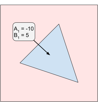
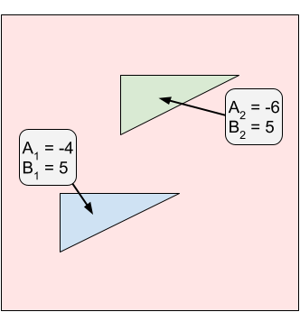
Today is your and your twin sibling's birthday. To celebrate, you got a rectangular cake to share. The cake is decorated with $$$\mathbf{N}$$$ triangular patches of icing (which may overlap). All the icing patches were created with the same triangular mold, so they have the same shape and orientation. Although you and your twin are very similar, your tastes in icing are much different. This difference is formalized by each of you having a different enjoyment value for each patch of icing. Specifically, your enjoyment value for eating the entire $$$i$$$-th patch of icing is $$$\mathbf{A_i}$$$, and your twin's is $$$\mathbf{B_i}$$$. If someone eats part of a patch, they get enjoyment proportional to the eaten area. For example, if you eat $$$\frac{2}{3}$$$ of the area of the $$$i$$$-th icing patch, you would get $$$\frac{2\mathbf{A_i}}{3}$$$ enjoyment from it. Note that there may be some flavors of icing that you or your twin do not enjoy, so the $$$\mathbf{A_i}$$$ and/or $$$\mathbf{B_i}$$$ values can be negative.
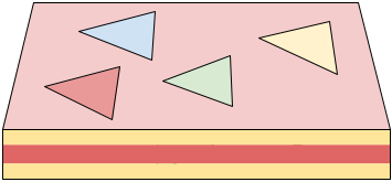
You will cut the cake into two rectangular pieces by making a single vertical cut (parallel to the Y-axis). After cutting the cake, you will eat the left piece and your twin will eat the right piece. Your total enjoyment is the sum of the enjoyment you get from all icing to the left of the cut. Similarly, your twin's enjoyment is the sum of the enjoyment they get from all icing to the right of the cut.
To be as fair as possible, you want to cut the cake such that the absolute value of the difference between your total enjoyment and your twin's total enjoyment is as small as possible. Given the $$$\mathbf{N}$$$ triangular icing patches on a rectangular cake, what is the minimum possible absolute value of the difference between your and your twin's total enjoyments you can get?
Input
The first line of the input gives the number of test cases, $$$\mathbf{T}$$$. $$$\mathbf{T}$$$ test cases follow. Each test case starts with a line containing three positive integers, $$$\mathbf{N}$$$, $$$\mathbf{W}$$$, and $$$\mathbf{H}$$$, representing the number of icing patches on the cake and the width and height of the top of the cake, respectively. The bottom-left corner of the cake is located at $$$(0, 0)$$$ and the top-right corner is at $$$(\mathbf{W}, \mathbf{H})$$$. Then, a line describing the icing patch mold follows. This line contains four integers: $$$\mathbf{P}$$$, $$$\mathbf{Q}$$$, $$$\mathbf{R}$$$, and $$$\mathbf{S}$$$. The icing patch mold is a triangle with vertices at $$$(0, 0)$$$, $$$(\mathbf{P}, \mathbf{Q})$$$, and $$$(\mathbf{R}, \mathbf{S})$$$. Then, $$$\mathbf{N}$$$ lines follow. The $$$i$$$-th of these lines contains four integers $$$\mathbf{X_i}$$$, $$$\mathbf{Y_i}$$$, $$$\mathbf{A_i}$$$, and $$$\mathbf{B_i}$$$. The $$$i$$$-th patch is a triangle with vertices at $$$(\mathbf{X_i}, \mathbf{Y_i})$$$, $$$(\mathbf{X_i} + \mathbf{P}, \mathbf{Y_i} + \mathbf{Q})$$$, and $$$(\mathbf{X_i} + \mathbf{R}, \mathbf{Y_i} + \mathbf{S})$$$. You would get $$$\mathbf{A_i}$$$ enjoyment from eating it and your twin would get $$$\mathbf{B_i}$$$ enjoyment.
Output
For each test case, output one line containing Case #$$$x$$$: $$$y$$$/$$$z$$$,
where $$$x$$$ is the test case number (starting from 1) and $$$\frac{y}{z}$$$ is the minimum
absolute value of the difference between your and your twin's total enjoyment that can be achieved
with a single vertical cut as an irreducible fraction (that is, $$$z$$$ must be positive and of
minimum possible value).
Limits
Time limit: 45 seconds.
Memory limit: 1 GB.
Test Set 1 (Visible Verdict)
$$$1 \le \mathbf{T} \le 100$$$.
$$$1 \le \mathbf{N} \le 100$$$.
$$$3 \le \mathbf{W} \le 10^9$$$.
$$$3 \le \mathbf{H} \le 10^9$$$.
$$$-10^9 \le \mathbf{A_i} \le 10^9$$$, for all $$$i$$$.
$$$-10^9 \le \mathbf{B_i} \le 10^9$$$, for all $$$i$$$.
$$$0 \le \mathbf{P} \le 10^9$$$.
$$$-10^9 \le \mathbf{Q} \le 10^9$$$.
$$$0 \le \mathbf{R} \le 10^9$$$.
$$$-10^9 \le \mathbf{S} \le 10^9$$$.
The three vertices of the mold $$$(0, 0)$$$, $$$(\mathbf{P}, \mathbf{Q})$$$, and $$$(\mathbf{R}, \mathbf{S})$$$
are not collinear.
The three vertices of each triangular icing patch are strictly inside the cake's borders.
Formally:
$$$1 \le \mathbf{X_i} \le \mathbf{W} - \max(\mathbf{P}, \mathbf{R}) - 1$$$, for all $$$i$$$, and
$$$\max(0, -\mathbf{Q}, -\mathbf{S}) + 1 \le \mathbf{Y_i} \le \mathbf{H} - \max(0, \mathbf{Q}, \mathbf{S}) - 1$$$, for all $$$i$$$.
Sample
4
1 5 5
3 -1 2 2
1 2 -10 5
2 100000000 50000000
80000000 0 40000000 40000000
5000001 2500000 500 -501
15000000 5000000 501 -400
2 10 10
0 2 4 2
2 2 -4 5
4 6 -6 5
3 622460462 608203753
486076103 36373156 502082214 284367873
98895371 126167607 823055173 -740793281
26430289 116311281 -398612375 -223683435
46950301 278229490 766767410 -550292032
Case #1: 5/1
Case #2: 288309900002019999899/320000000000000000
Case #3: 37/4
Case #4: 216757935773010988373334129808263414106891/187470029508637421883991794137967
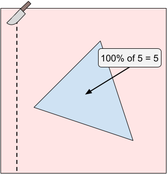
In Sample Case #1, there is a single icing patch. The optimal cut is to the left of the patch. You will eat no icing and receive $$$0$$$ enjoyment. Your twin will eat all of the icing patch and receive $$$5$$$ enjoyment from it. The absolute value of the difference between your and your twin's enjoyments is $$$|0 - 5| = 5$$$.
In Sample Case #2, there are two icing patches. The optimal cut is at $$$X = 15099999.99$$$. Notice that the numerator and denominator of the answer can get very large.
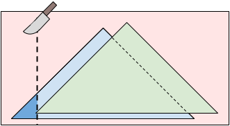
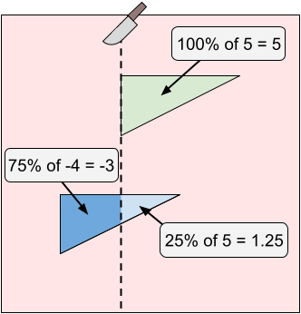
In Sample Case #3, there are two icing patches. The optimal cut is at $$$X = 4$$$. You will eat 75% of the first icing patch and receive $$$-3$$$ enjoyment from it. Your twin will eat 25% of the first icing patch and all of the second icing patch getting $$$5 \cdot 0.25 + 5 = 6.25$$$ enjoyment. The absolute value of the difference between your and your twin's enjoyments is $$$|-3 - 6.25| = 9.25 = \frac{37}{4}$$$.
Notice that cutting at $$$X = 1$$$ would give you $$$0$$$ enjoyment and your twin $$$10$$$ enjoyment. While both of those values are greater than the corresponding enjoyment when cutting at $$$X = 4$$$, the difference between them is $$$10 \gt 9.25$$$, which means cutting at $$$X = 4$$$ is preferable anyway.
In Sample Case #4, there are three icing patches. The optimal cut is at $$$X \approx 521241077.6027$$$.
B. Slide Circuits
Problem
Gooli is a huge company that owns $$$\mathbf{B}$$$ buildings in a hilly area. Five years ago, Gooli built slides that allowed employees to go from one building to another (they are not bidirectional), starting a tradition of building slides between buildings. Currently, $$$\mathbf{S}$$$ slides exist.
Melek is Gooli's Head of Transportation and a problem-solving enthusiast. She was tasked with keeping the slides enjoyable to use. The idea she came up with was disabling some slides such that only circuits remained. A circuit is a set of two or more buildings $$$b_1, b_2, ..., b_k$$$ such that there is exactly one slide enabled from building $$$b_i$$$ to building $$$b_{i+1}$$$, for each $$$i$$$, and exactly one slide enabled from building $$$b_k$$$ to building $$$b_1$$$. No other slides from or to any of those buildings should be enabled, to prevent misdirection. A state of the slides is then called fun if each building belongs to exactly one circuit.
Slides in Gooli's campus are numbered with integers between 1 and $$$\mathbf{S}$$$, inclusive. Melek created a slide controlling console that supports two operations: enable and disable. Both operations receive three parameters $$$\ell$$$, $$$r$$$, and $$$m$$$ and perform the operation on each slide $$$x$$$ such that $$$\ell \le x \le r$$$ and $$$x$$$ is a multiple of $$$m$$$. An enable operation is valid only if all affected slides are in a disabled state right before the operation is performed. Similarly, a disable operation is valid only if all affected slides are in an enabled state right before the operation is performed.
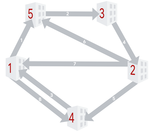
The following picture illustrates a possible succession of states and operations. The layout has $$$3$$$ buildings and $$$3$$$ slides. Slides are light grey when disabled and dark grey when enabled.
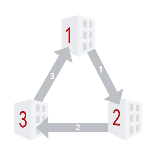
1. Initial state. All sides are disabled.
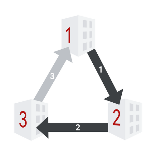
2. After enable operation with $$$\ell=1$$$, $$$r=2$$$, and $$$m=1$$$.
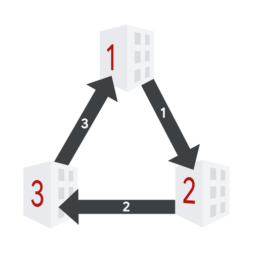
3. After enable operation with $$$\ell=3$$$, $$$r=3$$$, and $$$m=1$$$.
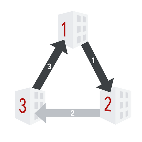
4. After disable operation with $$$\ell=1$$$, $$$r=3$$$, and $$$m=2$$$.
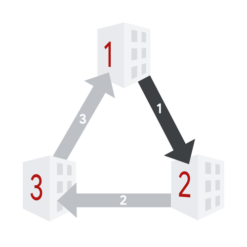
5. After disable operation with $$$\ell=1$$$, $$$r=3$$$, and $$$m=3$$$.
6. After enable operation with $$$\ell=1$$$, $$$r=2$$$, and $$$m=2$$$.
Unfortunately, Sult, Melek's cat, found the console and started performing several valid enable and disable operations. After every console operation performed by Sult, Melek wants to know if the state of the slides can be made fun by enabling exactly one currently disabled slide. Note that Melek does not actually enable this slide.
In the picture above, we can see that after the first, third, and last operations, Melek could enable the only disabled slide and get to a fun state. After the second operation, there are two issues. One issue is that there are no currently disabled slides, so Melek cannot enable any. Additionally, the state is already fun, so even if there were additional disabled slides, enabling anything would result in a not fun state. After the fourth operation, there are two disabled slides, but enabling either would not yield a fun state.
All slides are initially disabled, then Sult performs its operations one at a time. After each of Sult's operations, determine which disabled slide, if any, Melek can enable to put the slides in a fun state.
Input
The first line of the input gives the number of test cases, $$$\mathbf{T}$$$. $$$\mathbf{T}$$$ test cases follow.
Each test case starts with a line containing three integers $$$\mathbf{B}$$$, $$$\mathbf{S}$$$, and $$$\mathbf{N}$$$: the
number of buildings, slides, and operations to process, respectively.
Then, $$$\mathbf{S}$$$ lines follow. The $$$i$$$-th of these lines contains two integers
$$$\mathbf{X_i}$$$ and $$$\mathbf{Y_i}$$$, indicating that the slide with number $$$i$$$ goes from
building $$$\mathbf{X_i}$$$ to building $$$\mathbf{Y_i}$$$.
Finally, $$$\mathbf{N}$$$ lines represent the operations. The $$$j$$$-th of these lines
contains a character $$$\mathbf{A_j}$$$ and three integers $$$\mathbf{L_j}$$$, $$$\mathbf{R_j}$$$, and $$$\mathbf{M_j}$$$, describing
the $$$j$$$-th operation. $$$\mathbf{A_j}$$$ describes the type of operation using
an uppercase E for enable and an uppercase D for disable.
The operation is to be performed on slides with numbers that are simultaneously
a multiple of $$$\mathbf{M_j}$$$ and between $$$\mathbf{L_j}$$$ and $$$\mathbf{R_j}$$$, inclusive.
Output
For each test case, output one line containing
Case #$$$x$$$: $$$y_1\ y_2\ \dots\ y_\mathbf{N}$$$,
where $$$x$$$ is the test case number (starting from 1) and $$$y_j$$$ is an uppercase
X if there is no way to turn the state
of slides created by the first $$$j$$$ console operations into a fun state by enabling
exactly one disabled slide. Otherwise, $$$y_j$$$ should be an integer representing that
enabling the $$$y_j$$$-th slide would turn the state created by the first $$$j$$$ console operations
into a fun state.
Limits
Memory limit: 1 GB.
$$$1 \le \mathbf{X_i} \le \mathbf{B}$$$, for all $$$i$$$.
$$$1 \le \mathbf{Y_i} \le \mathbf{B}$$$, for all $$$i$$$.
$$$\mathbf{X_i} \ne \mathbf{Y_i}$$$, for all $$$i$$$.
$$$(\mathbf{X_i}, \mathbf{Y_i}) \neq (\mathbf{X_j}, \mathbf{Y_j})$$$, for all $$$i \neq j$$$.
$$$\mathbf{A_j}$$$ is either uppercase E or uppercase D, for all $$$j$$$.
$$$1 \le \mathbf{L_j} \le \mathbf{R_j} \le \mathbf{S}$$$, for all $$$j$$$.
$$$1 \le \mathbf{M_j} \le \mathbf{S}$$$, for all $$$j$$$.
Each operation is valid.
Test Set 1 (Visible Verdict)
Time limit: 10 seconds.
$$$1 \le \mathbf{T} \le 100$$$.
$$$2 \le \mathbf{B} \le 100$$$.
$$$2 \le \mathbf{S} \le 1000$$$.
$$$1 \le \mathbf{N} \le 1000$$$.
Test Set 2 (Hidden Verdict)
Time limit: 120 seconds.
$$$1 \le \mathbf{T} \le 30$$$.
$$$2 \le \mathbf{B} \le 3 \times 10^4$$$.
$$$2 \le \mathbf{S} \le 3 \times 10^5$$$.
$$$1 \le \mathbf{N} \le 3 \times 10^5$$$.
Sample
2
3 3 5
1 2
2 3
3 1
E 1 2 1
E 3 3 1
D 1 3 2
D 1 3 3
E 1 2 2
5 8 10
1 5
5 3
4 1
3 2
2 4
2 5
2 1
1 4
E 1 8 2
D 4 8 2
E 3 5 1
E 1 1 3
E 1 1 1
E 5 8 2
D 1 8 3
D 5 8 4
D 4 5 1
E 3 4 1
Case #1: 3 X 2 X 3
Case #2: 3 X 1 1 X X X 3 X 5
Sample Case #1 is the one depicted in the problem statement.
The following picture shows the building and slide layout of Sample Case #2.
The sets of enabled slides after each operation are:
- $$$\{2,4,6,8\}$$$,
- $$$\{2\}$$$,
- $$$\{2,3,4,5\}$$$,
- $$$\{2,3,4,5\}$$$,
- $$$\{1,2,3,4,5\}$$$,
- $$$\{1,2,3,4,5,6,8\}$$$,
- $$$\{1,2,4,5,8\}$$$,
- $$$\{1,2,4,5\}$$$,
- $$$\{1,2\}$$$, and
- $$$\{1,2,3,4\}$$$.
C. Ropes
Problem
Two scout teams are taking part in a scouting competition. It is the finals and each team is well prepared. The game is played along a river that flows west to east. There are $$$4\mathbf{N}$$$ trees planted along the river, with exactly $$$2\mathbf{N}$$$ of them lined up along the north bank and $$$2\mathbf{N}$$$ lined up along the south bank. Both teams alternate turns playing the game. Your team goes first.
On each turn, the playing team selects one tree on each bank that does not have any ropes tied to it and ties a rope between both trees, making it cross the river. Each rope that is added is placed higher than all previous ropes. The playing team scores 1 point per each previously used rope that passes below the newly added rope.
After $$$2\mathbf{N}$$$ turns, all trees have exactly one rope tied to them, so there are no more possible plays and the game is over. The score of each team is the sum of the scores they got in all of their turns. If your team's score is strictly greater than the opposing team's score, your team wins. If your team's score is less than or equal to the opposing team's score, your team does not win.
The following animation shows a possible game with $$$\mathbf{N}=2$$$. Your team is represented by the color red and the other team by the color blue.
The opposing team felt confident that going second is a large advantage, so they revealed their strategy. On their turn, they choose the play that yields the maximum possible score for this turn. If multiple such plays exist, they choose one at random. This choice is generated uniformly at random, and independently for each play, for each test case and for each submission. Therefore, even if you submit exactly the same code twice, the opposing team can make different random choices.
You play $$$\mathbf{T}$$$ games in total, and your team must win at least $$$\mathbf{W}$$$ of them.
Input and output
This is an interactive problem. You should make sure you have read the information in the Interactive Problems section of our FAQ.
Initially, your program should read a single line containing three integers $$$\mathbf{T}$$$, $$$\mathbf{N}$$$, and $$$\mathbf{W}$$$: the number of test cases, the number of turns of your team and the number of wins you need to get for your solution to be considered correct, respectively. Note that the opposing team also gets $$$\mathbf{N}$$$ turns, for a total of $$$2\mathbf{N}$$$ turns for each test case.
For each test case, your program must process $$$\mathbf{N}$$$ exchanges. Each exchange represents two consecutive turns, one from your team and one from the opposing team.
For the $$$i$$$-th exchange, you must first print a single line with two integers $$$\mathbf{A_i}$$$ and $$$\mathbf{B_i}$$$ and then read a single line with two integers $$$\mathbf{C_i}$$$ and $$$\mathbf{D_i}$$$. This represents that in your $$$i$$$-th turn you tied the rope between the $$$\mathbf{A_i}$$$-th tree from the west on the north bank and the $$$\mathbf{B_i}$$$-th tree from the west on the south bank. Similarly, in the opposing team's $$$i$$$-th turn they used the $$$\mathbf{C_i}$$$-th tree from the west on the north bank and the $$$\mathbf{D_i}$$$-th tree from the west on the south bank. Trees are indexed starting from 1.
After the $$$\mathbf{N}$$$ exchanges, you must read one number that represents the result of this game. This number will be 1 if your team won, otherwise it will be 0.
The next test case starts immediately if there is one. If this was the last test case, the judge will expect no more output and will send no further input to your program. In addition, all $$$\mathbf{T}$$$ test cases are always processed, regardless of whether it is already guaranteed that the threshold for correctness will or cannot be met. The threshold is only checked after correctly processing all test cases.
If the judge receives an invalidly formatted line or invalid move (like using a tree that has already been used) from your program at any moment, the judge will print a single number -1 and will not print any further output. If your program continues to wait for the judge after receiving a -1, your program will time out, resulting in a Time Limit Exceeded error. Notice that it is your responsibility to have your program exit in time to receive a Wrong Answer judgment instead of a Time Limit Exceeded error. As usual, if the memory limit is exceeded, or your program gets a runtime error, you will receive the appropriate judgment.
Limits
Time limit: 90 seconds.
Memory limit: 1 GB.
$$$\mathbf{T} = 2000$$$.
$$$\mathbf{N} = 50$$$.
Test Set 1 (Visible Verdict)
$$$\mathbf{W} = 1200$$$ ($$$\mathbf{W} = 0.6 \cdot \mathbf{T}$$$).
Test Set 2 (Visible Verdict)
$$$\mathbf{W} = 1560$$$ ($$$\mathbf{W} = 0.78 \cdot \mathbf{T}$$$).
Test Set 3 (Visible Verdict)
$$$\mathbf{W} = 1720$$$ ($$$\mathbf{W} = 0.86 \cdot \mathbf{T}$$$).
Testing Tool
You can use this testing tool to test locally or on our platform. To test locally, you will need to run the tool in parallel with your code; you can use our interactive runner for that. For more information, read the instructions in comments in that file, and also check out the Interactive Problems section of the FAQ.
Instructions for the testing tool are included in comments within the tool. We encourage you to add your own test cases. Please be advised that although the testing tool is intended to simulate the judging system, it is NOT the real judging system and might behave differently. If your code passes the testing tool but fails the real judge, please check the Coding section of the FAQ to make sure that you are using the same compiler as us.
2 2 1
3 2
4 1
1 3
2 4
0
1 1
2 3
3 2
4 4
1
D. Divisible Divisions
Problem
We have a string $$$\mathbf{S}$$$ consisting of decimal digits. A division of $$$\mathbf{S}$$$ is created by
dividing $$$\mathbf{S}$$$ into contiguous substrings.
For example, if $$$\mathbf{S}$$$ is 0145217, two possible divisions are
014 5 21 7 and 0 14 52 17. Each digit must be used in exactly one
substring, and each substring must be non-empty. If $$$\mathbf{S}$$$ has $$$L$$$ digits, then there are exactly
$$$2^{L-1}$$$ possible divisions of it.
Given a positive integer $$$\mathbf{D}$$$, a division of $$$\mathbf{S}$$$ is called divisible by $$$\mathbf{D}$$$ if for every
pair of consecutive substrings, at least one of the integers they represent in base $$$10$$$
is divisible by $$$\mathbf{D}$$$.
If $$$\mathbf{D}=7$$$, the first example division above is divisible because 014,
21, and 7 represent integers divisible by $$$7$$$. The second example
division is not divisible because 52 and 17 are consecutive substrings
and neither represents an integer divisible by $$$7$$$. Dividing 0145217 as
0145217 is divisible by any $$$\mathbf{D}$$$ because there are no pairs of consecutive substrings.
Given $$$\mathbf{S}$$$ and $$$\mathbf{D}$$$, count how many divisions of $$$\mathbf{S}$$$ exist that are divisible by $$$\mathbf{D}$$$. Since the output can be a really big number, we only ask you to output the remainder of dividing the result by the prime $$$10^9+7$$$ ($$$1000000007$$$).
Input
The first line of the input gives the number of test cases, $$$\mathbf{T}$$$. $$$\mathbf{T}$$$ lines follow. Each line represents a test case with a string of digits $$$\mathbf{S}$$$ and a positive integer $$$\mathbf{D}$$$, as mentioned above.
Output
For each test case, output one line containing Case #$$$x$$$: $$$y$$$,
where $$$x$$$ is the test case number (starting from 1) and $$$y$$$ is the number of
different divisions of $$$\mathbf{S}$$$ that are divisible by $$$\mathbf{D}$$$, modulo the prime
$$$10^9+7$$$ ($$$1000000007$$$).
Limits
Time limit: 60 seconds.
Memory limit: 1 GB.
$$$1 \le \mathbf{T} \le 100$$$.
$$$1 \le \mathbf{D} \le 10^6$$$.
Test Set 1 (Visible Verdict)
$$$1 \le $$$ the length of $$$\mathbf{S} \le 1000$$$.
Test Set 2 (Hidden Verdict)
$$$1 \le $$$ the length of $$$\mathbf{S} \le 10^5$$$.
Sample
3
0145217 7
100100 10
5555 12
Case #1: 16
Case #2: 30
Case #3: 1
In Sample Case #1, all $$$16$$$ divisible divisions of $$$\mathbf{S}$$$ are:
0145217,0 145217,0 14 5217,0 14 5 217,0 14 5 21 7,0 14 521 7,0 145 217,0 145 21 7,0 14521 7,014 5217,014 5 217,014 5 21 7,014 521 7,0145 217,0145 21 7, and014521 7.
In Sample Case #2, there are $$$2^5=32$$$ ways to divide in total. To get two consecutive
substrings to not be divisible by $$$10$$$, we need both of them to not end in $$$0$$$. The
only $$$2$$$ ways of doing that are 1 001 00 and 1 001 0 0, which
means the other $$$30$$$ divisions of $$$\mathbf{S}$$$ are divisible by $$$10$$$.
In Sample Case #3, no possible substring represents an even integer, which in turn means
it is not divisible by $$$12$$$. Therefore, the only way to not have two consecutive substrings
that are not divisible by $$$12$$$ is to not have two consecutive substrings at all, which
can be done in only $$$1$$$ way: 5555.
E. Infinitree
Problem
This problem is about finding the distance between two nodes of a strictly binary tree. Oh, is that too easy?! Ok, the tree is potentially infinite now. Keep it up and we will start going up the aleph numbers.
In this problem, a tree is either a single node $$$X$$$, or a node $$$X$$$ with two trees attached to it: a left subtree and a right subtree. In both cases, $$$X$$$ is the root of the tree. If the tree is not a single node, the roots of both the left and right subtrees are the only children of $$$X$$$.
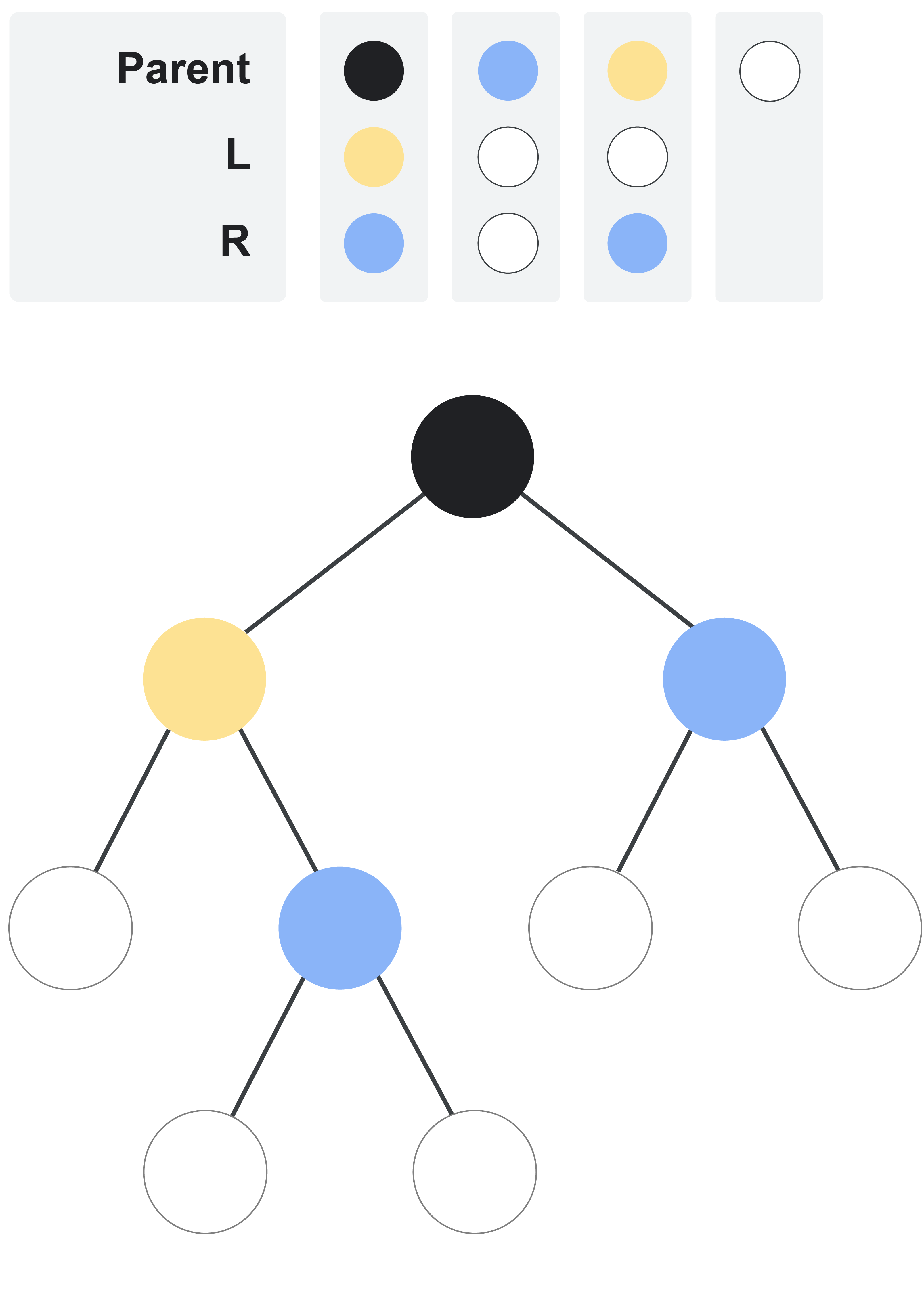
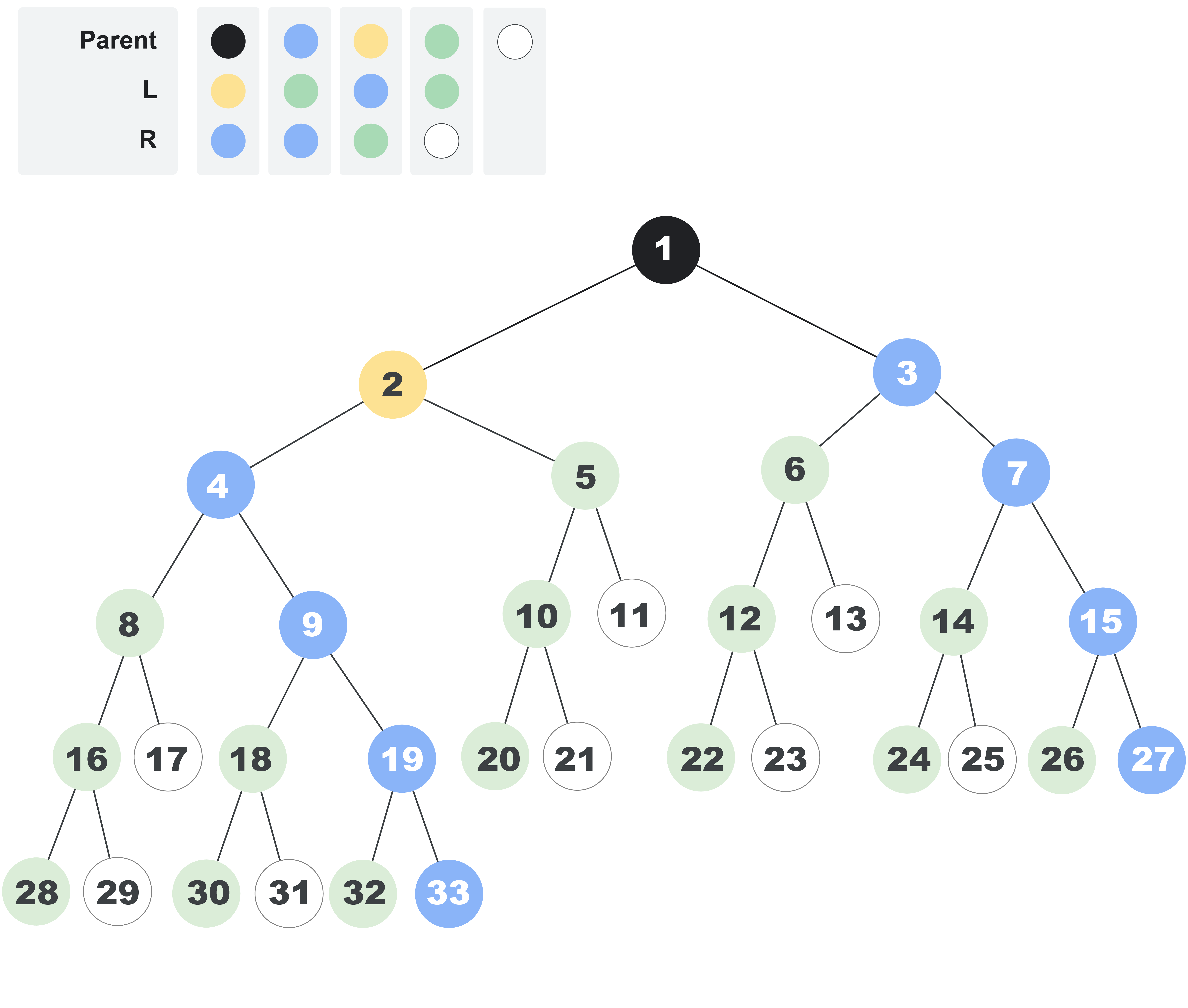
There is a set of colors numbered from $$$0$$$ to $$$\mathbf{N}$$$, inclusive. Each node is of exactly one color. There might be zero, one, or multiple nodes of each color. Each node of color $$$0$$$ (white) is a leaf node (that is, it has no children). Each node of color $$$i$$$, for $$$1 \le i \le \mathbf{N}$$$, has exactly $$$2$$$ children: the left one is color $$$\mathbf{L_i}$$$ and the right one is color $$$\mathbf{R_i}$$$. The root of the tree is color $$$1$$$ (black). Note that the tree may have a finite or countably infinite number of nodes.
For example, the following picture illustrates a finite tree defined by the lists $$$\mathbf{L} = [3, 0, 0]$$$ and $$$\mathbf{R} = [2, 0, 2]$$$. Color $$$2$$$ is blue and color $$$3$$$ is yellow.
The distance between two nodes in the tree is the minimum number of steps that are needed to get from one node to the other. A step is a move from a node to its direct parent or its direct child.
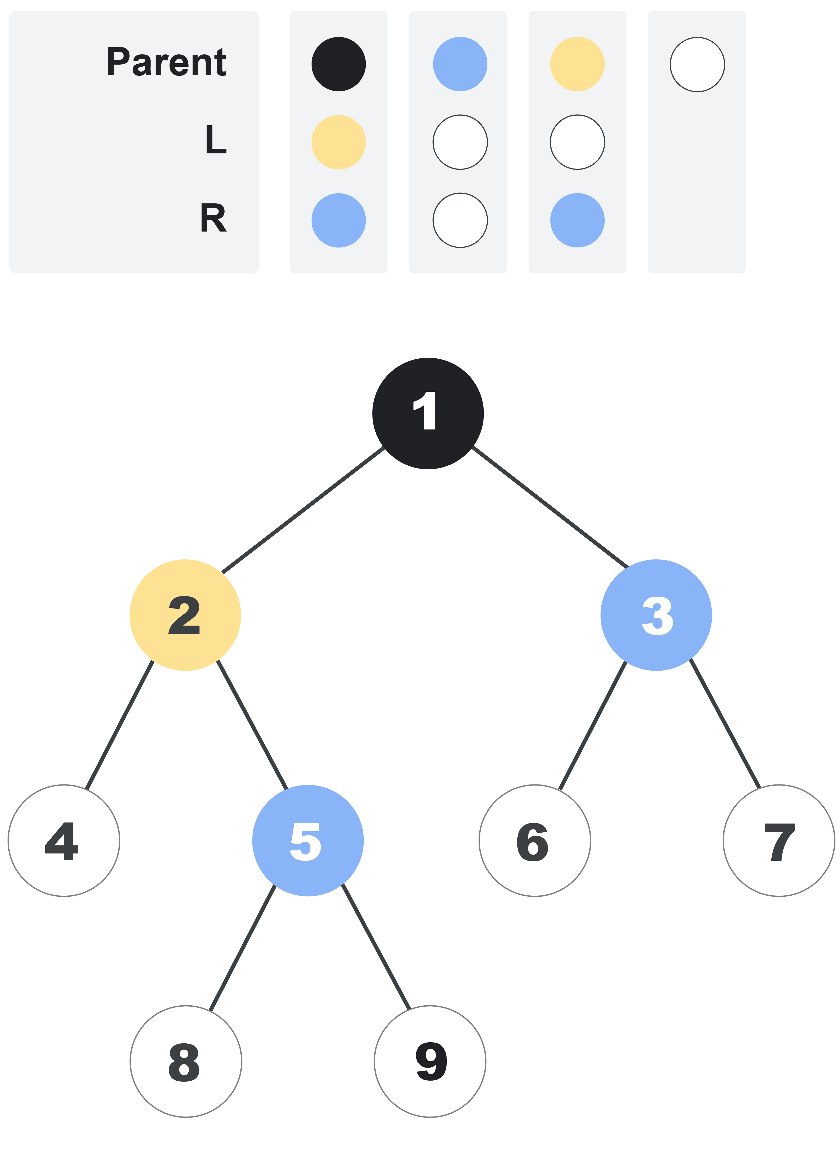
Nodes in the tree are indexed using positive integers. The root has index $$$1$$$. Then, other nodes are indexed using consecutive integers, with nodes with smaller distances to the root being indexed first. For nodes that are equidistant to the root, nodes that are further to the left are indexed first. For example, the following picture adds indices to each node in the tree we presented before. Notice that each node's index is independent from its color.
As another example, the following picture shows the first $$$33$$$ nodes of an infinite tree defined by the lists $$$\mathbf{L} = [3, 4, 2, 4]$$$ and $$$\mathbf{R} = [2, 2, 4, 0]$$$. Color $$$4$$$ is green.
Given the lists $$$\mathbf{L}$$$ and $$$\mathbf{R}$$$ that define a tree and the indices of two different nodes in the tree, return the distance between those two nodes.
Input
The first line of the input gives the number of test cases, $$$\mathbf{T}$$$. $$$\mathbf{T}$$$ test cases follow. Each test case consists of three lines. The first line contains $$$\mathbf{N}$$$, $$$\mathbf{A}$$$, and $$$\mathbf{B}$$$: the size of the lists that define the tree, and the indices of the two nodes whose distance you need to calculate, respectively. The second line contains $$$\mathbf{N}$$$ integers $$$\mathbf{L_1}, \mathbf{L_2}, \dots, \mathbf{L_N}$$$ and the third line contains $$$\mathbf{N}$$$ integers $$$\mathbf{R_1}, \mathbf{R_2}, \dots, \mathbf{R_N}$$$, as described above.
Output
For each test case, output one line containing Case #$$$x$$$: $$$y$$$,
where $$$x$$$ is the test case number (starting from 1) and $$$y$$$ is
the distance between the nodes with indices $$$\mathbf{A}$$$ and $$$\mathbf{B}$$$ in the tree defined by the lists $$$\mathbf{L}$$$
and $$$\mathbf{R}$$$.
Limits
Time limit: 90 seconds.
Memory limit: 1 GB.
$$$1 \le \mathbf{T} \le 100$$$.
$$$1 \le \mathbf{N} \le 50$$$.
$$$0 \le \mathbf{L_i} \le \mathbf{N}$$$.
$$$0 \le \mathbf{R_i} \le \mathbf{N}$$$.
$$$\mathbf{A} \lt \mathbf{B} \le 10^{18}$$$.
The tree defined by $$$\mathbf{L}$$$ and $$$\mathbf{R}$$$ has at least $$$\mathbf{B}$$$ nodes.
Test Set 1 (Visible Verdict)
$$$\mathbf{A} = 1$$$.
Test Set 2 (Hidden Verdict)
$$$1 \le \mathbf{A} \le 10^{18}$$$.
Sample
Note: there are additional samples that are not run on submissions down below.5 3 1 8 3 0 0 2 0 2 3 1 5 3 0 0 2 0 2 4 1 27 3 4 2 4 2 2 4 0 4 1 28 3 4 2 4 2 2 4 0 3 1 10 1 3 1 3 2 1
Case #1: 3
Case #2: 2
Case #3: 4
Case #4: 5
Case #5: 3
The tree in Sample Cases #1 and #2 is the first tree shown in the statement. The tree in Sample Cases #3 and #4 is the last tree shown in the statement. The same is true for the additional samples below. In Sample Case #5, notice that some colors may not be present in the tree.
Additional Sample - Test Set 2
The following additional sample fits the limits of Test Set 2. It will not be run against your submitted solutions.4 3 5 7 3 0 0 2 0 2 3 4 9 3 0 0 2 0 2 4 11 18 3 4 2 4 2 2 4 0 4 21 22 3 4 2 4 2 2 4 0
Case #1: 4
Case #2: 3
Case #3: 5
Case #4: 8
Analysis — A. Cutting Cake
A Single Icing Patch
Let's first consider a case where we have only one icing patch with a vertical edge on the right having enjoyment values $$$\mathbf{A}$$$ and $$$\mathbf{B}$$$. If our vertical cut line is all the way to the left of the triangle, we would get $$$0$$$ enjoyment and our twin would get $$$\mathbf{B}$$$ enjoyment. If our cut line is to the right of the triangle, we would get $$$\mathbf{A}$$$ enjoyment and our twin would get $$$0$$$ enjoyment.
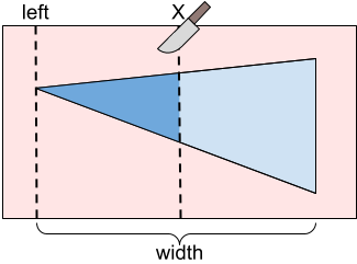
Otherwise, our cut is somewhere in the middle of the triangle. In this case, we would get $$$\mathbf{A} \cdot P(X)$$$ enjoyment and our twin would get $$$\mathbf{B} \cdot (1 - P(X))$$$ enjoyment where $$$P(X)$$$ is a value between 0 and 1 representing the proportion of the triangle that is to the left of a cut line at position $$$X$$$.
We can calculate $$$P(X)$$$ by considering similar triangles. Let $$$T_X$$$ be the triangle that is to the left of our cut line when cutting at $$$X$$$. We can notice that $$$T_X$$$ and our full triangle are similar triangles. This means that the ratio between the width and height of $$$T_X$$$ is the same as the ratio for the full triangle. So, given a cut location $$$X$$$, the width and height of $$$T_X$$$ are both $$$\frac{X - \text{left}}{\text{width}}$$$ of the full triangle's width and height respectively. Therefore, we can calculate $$$P(X)$$$ using the following formula:
$$$$P(X) = \left(\frac{X - \text{left}}{\text{width}} \right) ^2$$$$
Notice that $$$P(X)$$$ is a quadratic (polynomial of degree 2). With this, we can write the formulas for our enjoyment and our twin's enjoyment as polynomials in terms of $$$X$$$:
$$$$\text{Our enjoyment} = \mathbf{A} \cdot \left(\frac{X - \text{left}}{\text{width}} \right) ^2$$$$ $$$$\text{Twin's enjoyment} = \mathbf{B} \cdot \left(1 - \left(\frac{X - \text{left}}{\text{width}} \right) ^2\right)$$$$
The value we care about is the difference between these enjoyments. So, we can take the difference between enjoyments and solve for the minimum absolute value within a given range of our cut X-coordinate (from the left of the triangle to the right of the triangle). We can do this by checking the following:
- The value at the extreme point of the quadratic, if that's within the interval.
- The values at each endpoint of the interval.
- Whether the quadratic crosses 0 within the interval.
We can know whether the function crosses $$$0$$$ by checking whether the sign at the two endpoints is different. In case the extreme value is within the range, we need to check whether that sign is different from endpoints as well.
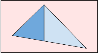
Note that our triangle mold might not have a vertical edge. In this case, we can split the triangle in two parts and solve for the left and right sides separately.
The formula for the right side is slightly different but very similar to that used for the left. So, we can calculate the proportion, $$$P(X)$$$, for a triangle with a vertical edge on the left as follows:
$$$$P(X) = 1 - \left(\frac{\text{left} + \text{width} - X}{\text{width}} \right) ^2$$$$
Many Icing Patches
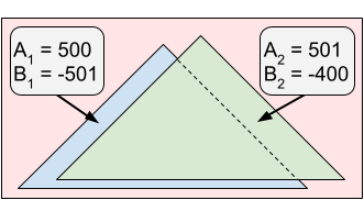
For the full problem, we have many icing patches. If we look at all unique X-coordinates of the vertices representing the triangular icing patches, we can notice that if we cut somewhere between two adjacent X-coordinates, each triangle is either always:
- Entirely to the left of our cut line (contributing to our enjoyment).
- Entirely to the right of our cut line (contributing to our twin's enjoyment).
- Cut in two pieces by the cut line (contributing to both our and our twin's enjoyment).
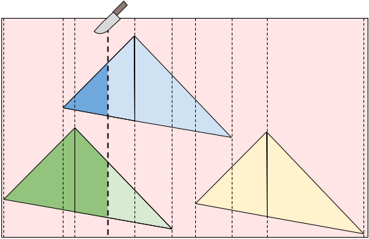
Therefore, for every pair of adjacent X-coordinates, we can add the constant enjoyments from the triangles that are always either to the left or to the right of the cut line to the quadratic functions from the triangles that are being cut. This means that the function $$$D(X)$$$ that represents the difference between enjoyments if we cut at $$$X$$$ is a piece-wise polynomial of degree no more than two. Between every pair of adjacent X-coordinates, we can solve for the minimum absolute value of the difference between our and our twin's enjoyment. Our final answer is then the minimum across all X-coordinate ranges.
Using a sweep-line technique, we can maintain the polynomials representing our and our twin's enjoyments. Because we need to sort the points by X-coordinate, our overall solution requires $$$O(\mathbf{N} \log \mathbf{N})$$$ operations for sorting and $$$O(\mathbf{N})$$$ operations on fractions. Keep in mind that the numbers for the numerator and denominator might not fit into 64 bit integers. Notice that the size of those numbers grows logarithmically in the size of the input, so $$$O(\mathbf{N} \log \mathbf{N})$$$ operations is a reasonable approximation of the overall time complexity of the algorithm.
Some behind the scenes trivia
Because of the $$$O(\mathbf{N} \log \mathbf{N})$$$ complexity mentioned in the previous paragraph, this problem started out as the same statement but intended to be solved using floating point. However, as illustrated by the fact that it needs fractions with integers that do not fit in 128 bits, the precision was a big problem. The amount of restriction all variables needed to keep the precision issues workable would have made a solution that simply iterates through all triangles for every range and does a ternary search usable. Such a solution can be guessed without understanding the polynomials we explained. Using fractions was a way to require solutions to understand those polynomials. Setting a small value for $$$\mathbf{N}$$$ allows using unbounded integers without worrying about the additional running time. Making all the triangles the same shape also helps with this: it keeps the size of the fractions from getting too big.
Analysis — B. Slide Circuits
To simplify the notation, we can reframe this problem in terms of graphs. We represent the input with a graph $$$G$$$ that has one node per building and one directed edge per slide. The enabled/disabled states we can represent by subgraphs $$$G_1, G_2, ..., G_\mathbf{N}$$$ where $$$G_i$$$ is a subgraph of $$$G$$$ containing only the edges representing slides that are enabled after the first $$$i$$$ operations.
A graph is fun if every node belongs to exactly one cycle. The question is, for each $$$i$$$, to identify an edge $$$(v, w) \in G - G_i$$$ such that $$$G_i \cup \{(v, w)\}$$$ is fun.
Test Set 1
The first step to solve the problem is to describe fun graphs more directly: A graph is fun if the in-degree and out-degree of every node is $$$1$$$. Therefore, the edge $$$(v, w)$$$ that we need in step $$$i$$$ must be such that the out-degree of $$$v$$$ in $$$G_i$$$ is $$$0$$$, the in-degree of $$$w$$$ in $$$G_i$$$ is $$$0$$$ and all other in-degrees and out-degrees in $$$G_i$$$ are $$$1$$$. This implies that, given $$$G_i$$$, we can simply check the degrees and find the only possible candidate for $$$v$$$ and $$$w$$$, if any. If $$$(v, w) \in G$$$, we found a answer. If there is no candidate for either, or $$$(v, w) \not\in G$$$, then there is no answer for step $$$i$$$.
In Test Set 1, we can maintain the in-degree and out-degree of each node in the current $$$G_i$$$. When there is an enable operation, for each affected edge $$$(v, w)$$$ we need to increase the out-degree of $$$v$$$ and the in-degree of $$$w$$$ by $$$1$$$. For disable operations, we do the same but decreasing by $$$1$$$. Then, we can do a linear pass to find candidates $$$v$$$ and $$$w$$$. If there are unique candidates for both, we check if $$$(v, w)$$$ is in $$$G$$$ and give the appropriate output. This can be done in linear time in the size of the graph per step, which is $$$O(\mathbf{B} + \mathbf{S})$$$ time, or $$$O(\mathbf{N} (\mathbf{B} + \mathbf{S}))$$$ time overall, which is fast enough to pass Test Set 1.
Test Set 2
Our solution for Test Set 2 is an optimized version of the solution presented for Test Set 1. Consider multisets of nodes $$$I_i$$$ and $$$O_i$$$. The number of occurrences of $$$v$$$ in $$$I_i$$$ is equal to the out-degree of $$$v$$$ in $$$G_i$$$, and the number of occurrences of $$$v$$$ in $$$O_i$$$ is equal to the out-degree of $$$v$$$ in $$$G_i$$$. Let $$${I'}_e$$$ and $$${O'}_e$$$ be the way the multisets $$$I_i$$$ and $$$O_i$$$ should look for $$$e$$$ to be the answer after step $$$i$$$.
If we keep hashes of the $$$I_i$$$ and $$$O_i$$$ that are efficient to update and check a dictionary from the pairs of hashes of $$$({I'}_e, {O'}_e) \to e$$$, we can solve the problem. There are many options that work with different trade-offs in reliability, ease of implementation and ease of proof.
Sum of random values
Let us start by assigning a random integer $$$x_v$$$ to each vertex $$$v$$$, that we keep throughout a test case. The hash of a multiset in this case is the sum of the values over all the vertices it contains (if it contains a vertex multiple times, its value is summed that many times), modulo some large number. For extra randomness we could use separate values for the $$$I$$$ and $$$O$$$ hashes.
Let $$$t = \sum_v x_v$$$ be the sum of all those random values. Then, the hash of $$${I'}_{(v, w)}$$$ is simply $$$t - x_w$$$ and the hash of $$${O'}_{(v, w)}$$$ is $$$t - x_w$$$. To get the hashes of $$${I'}_{i+1}$$$ and $$${O'}_{i+1}$$$ we can add or subtract to the hashes of $$${I'}_i$$$ and $$${O'}_i$$$ (for simplicity, $$${I'}_0 = {O'}_0 = 0$$$). The amount to add or subtract is the sum of the values of the starting/ending points of all edges that the operation is changing. We can find that efficiently by building two arrays (one for starting points and one for ending points) of sums over the first $$$i$$$ multiples of $$$M$$$ for each $$$i$$$ and each $$$M$$$. Then, the sum between the $$$i$$$-th and $$$j$$$-th multiples of $$$M$$$ is just the difference between the values for $$$M,j$$$ and $$$M,i-1$$$. The array for a specific value of $$$M$$$ contains $$$\lfloor \mathbf{S} / M \rfloor$$$ values, and $$$\sum_{M \le \mathbf{S}} \lfloor \mathbf{S} / M \rfloor \le \sum_{M \le \mathbf{S}} \mathbf{S} / M = \mathbf{S} \sum_{M \le \mathbf{S}} 1 / M = O(\mathbf{S} \log \mathbf{S})$$$, so this is efficient enough.
It has hard to prove formally that the sums work well as hashes. We present next a closely related variant for which is much easier to be convinced that the probability of collisions is really small.
XOR of random values
The idea in this case is to use XOR instead of sum. The whole implementation can be done in the same way as in the previous case. However, because XOR is its own inverse, two multisets with the same parity in the number of occurrences for all vertices have the same hash. We can solve this by adding a count of the number of edges in $$$G_i$$$. This can still cause collisions, but since all numbers of occurrences in $$$I'$$$ and $$$O'$$$ are either $$$0$$$ or $$$1$$$, having both the correct parities and the correct total guarantees we are looking at the same multiset. This does require maintaining that total number of edges update, but that can be done in constant time per step.
In the case of XORs, each bit in the result is independent from all other bits. Since the values $$$x_v$$$ are randomized, the probability of the bit being equal in two multisets with different parities is $$$1/2$$$. Therefore, the probability of $$$64$$$ bits coinciding by chance is $$$2^{-64}$$$, which is vanishingly small.
Polynomial hashes
Finally, in the XOR version above, we are actually hashing sets of nodes depending on the parity of their in- or out-degree, in a way. We know polynomial hashes are good for hashing sets, so we can simply use one of them. This is a third way of solving the problem.
Notice that a polynomial hash is actually equivalent to the sum version except the $$$x_v$$$ values are powers of a prime instead of randomly chosen. Random choices are more resilient to adversary data and provide similar properties of uniformity of distribution. This is an informal argument that justifies the sum of random values being a good hashing for this problem.
Analysis — C. Ropes
This problem can be solved in many different ways! Below is a collection of different solutions we came across. If yours is not here, we would love to hear it! Head over to our Code Jam group and share your favorite idea.
For consistency, here are a few terms we will use throughout:
- "Playing $$$(x,y)$$$" means connecting tree $$$x$$$ on the North to tree $$$y$$$ on the South.
- "Playing greedily" means looking at all possible options and choosing a move that maximizes your score on this turn. Sometimes we will choose randomly, sometimes we will pick a specific one of these. Note that the judge plays greedily (and chooses their move randomly).
The percentages given below are approximate (found via experimentation) and rounded to the closest integer value.
Playing Greedily
... by picking randomly ($$$28\%$$$)
We just pick our move randomly like the opponent is going to. This is not a great strategy!
... by picking non-randomly ($$$55\%$$$)
This strategy works surprisingly well for how simple it is. Simply play the same way as your opponent, except instead of picking randomly, choose the one that comes first lexicographically—that is, choose $$$(x,y)$$$ that minimizes $$$x$$$, then minimizes $$$y$$$ if there is a tie. To understand why it works well, read the "Push Them East!" strategy, as they work for similar reasons.
... by picking non-randomly and starting in a better place
This the same as the previous strategy, but instead of starting at $$$(1,1)$$$, we pick some other spot. The result varies depending on the exact starting spot, but $$$(1,3)$$$ already gets us $$$75\%$$$ probability of winning. Read below to understand why this has such a big impact in the overall probability.
Mirroring
First attempt ($$$64\%$$$)
This strategy is based on a simple idea: if the opposing team plays $$$(x,y)$$$, then we will play $$$(y,x)$$$. Why is this a good idea? Because if they just played $$$(x,y)$$$ and scored $$$\Delta$$$ points, then we will score $$$\Delta + 1$$$ points on our turn because we will also cross their newly placed rope as well as all other ropes the opponent just crossed.
There are two issues, though. The first issue is that we are going first, so we cannot mirror them. We will solve this by playing $$$(1,1)$$$ as our first move. This move does not impact the remainder of the game as no other rope can cross this one. The second issue is what to do when they play $$$(x,x)$$$? In this case, we will just play the highest scoring $$$(z,z)$$$ that is available.
Now with a better start ($$$82\%$$$)
This strategy is the same as the previous section, except our first move is $$$(10,10)$$$ instead of $$$(1,1)$$$. Why is this better? Think about when we did well in the previous version. If $$$x \neq y$$$, then we gain one point on them. The only time they can gain on us is if $$$x = y$$$ (or it is their last turn). By playing $$$(10,10)$$$, we are encouraging them to play diagonal moves early on in the game, which gains us a reasonably good lead. 10 was found experimentally to be the best value. Starting with $$$(2,2)$$$ gives $$$72\%$$$ and starting with $$$(25,25)$$$ gives $$$64\%$$$.
Push It East!
First attempt ($$$50\%$$$)
It will help to think of this in three phases: Phase $$$1$$$ sets up the ropes in a reasonable way (and hopefully gains us some points). Phase $$$2$$$ plays greedily (and hopefully maintains the lead from Phase $$$1$$$). Phase $$$3$$$ is the final turn for our opponent (hopefully their score from this turn is small).
This strategy is called "Push It East!" because our main goal is to make Phase $$$3$$$ as bad as possible for our opponent, and how we do that is ensure that their final move is as far East as possible. If their final move is $$$(x,y)$$$, then the maximum they can possibly score is $$$(100-x) + (100-y)$$$. In particular, if we can push them all the way to the East, they will score 0.
For our first attempt, Phase $$$1$$$ will simply "give up" our first turn by playing $$$(1,1)$$$. We enter Phase $$$2$$$ now (note that we are currently tied). Phase $$$2$$$ will play greedily, breaking ties by taking more western trees as often as possible (say by choosing $$$(x,y)$$$ that minimizes $$$x + y$$$). With this setup, Phase $$$3$$$ will typically take a tree that is quite far East. (Yay!)
A better start ($$$73\%$$$)
If we start Phase $$$1$$$ with $$$(2,2)$$$, then the opponents will play $$$(1,x)$$$ (or $$$(x,1)$$$), scoring one point. We then play $$$(1,3)$$$ (or $$$(3,1)$$$), scoring two points. At this point, we enter Phase $$$2$$$ ahead by one point and the opponent can only score at most one point on the next turn. This dramatically improves our win probability.
A great start ($$$92\%$$$)
Let $$$z$$$ be an integer near 10 (say 9, 10, or 11). Let's start Phase $$$1$$$ with $$$(z,z)$$$. For the next few moves, the opponent's moves will typically be $$$(x,y)$$$, where one of $$$x$$$ and $$$y$$$ is "small" ($$$\lt z$$$) and the other is "large" ($$$\gt z$$$). We can continue encouraging the opponent to make these "small"/"large" moves by choosing moves that are "short" ($$$(x,y)$$$ or $$$(y,x)$$$ where $$$x \lt 10$$$, but as large as possible, and $$$y \gt 10$$$, but as small as possible). We will continue making "short" moves which further encourages the opponent making "small"/"large" moves.
Say $$$z = 10$$$. After we have made $$$10$$$ moves (and the opponent has made $$$9$$$), we should now be ahead by $$$5$$$ to $$$10$$$ points (since we score approximately $$$0+2+\cdots+18$$$ and they score approximately $$$1+3+5+\cdots+17$$$). Phase $$$2$$$ contains 90 greedy moves for each of us where we typically maintain the $$$5-10$$$ point lead. Then, in the opponent's final turn, we hope they score fewer than 5 points since we have pushed them so far East.
Notice that just choosing every move (except the first) to be $$$(x,y)$$$ that first maximizes the score, then minimizes $$$x + y$$$ as above also works quite well because maximum score moves will usually cross our $$$(z,z)$$$ rope. This gets win percentages around $$$92\%$$$ as well.
Analysis — D. Divisible Divisions
Test Set 1
In Test Set 1, $$$\mathbf{S}$$$ is reasonably small. This allows us to compute the answer for every prefix of the input using dynamic programming. We compute two values for every prefix ending at index $$$i$$$: $$$A_i$$$ and $$$B_i$$$, which are the number of divisible divisions of this prefix whose last division is divisible by $$$\mathbf{D}$$$ (Type A) and the number of divisible divisions of this prefix whose last division is not divisible by $$$\mathbf{D}$$$ (Type B). The empty prefix has corresponding values $$$A_0 = 1$$$ and $$$B_0 = 0$$$. The solution to the problem is $$$A_{\text{length}(\mathbf{S})} + B_{\text{length}(\mathbf{S})}$$$.
Let $$$\mathbf{S}[i..j]$$$ be the integer represented by the digits in $$$\mathbf{S}$$$ from index $$$i$$$ to index $$$j$$$, inclusive. If $$$i > j$$$, then this is an empty substring and the corresponding value is $$$0$$$ (this only happens with $$$j=0$$$ below). To compute $$$A_k$$$, we will iterate over all possible last divisions ($$$\mathbf{S}[1..k], \mathbf{S}[2..k], \dots, \mathbf{S}[(k-1)..k], \mathbf{S}[k..k]$$$). For each one of these substrings (say $$$\mathbf{S}[i..k]$$$), we check if it is divisible by $$$\mathbf{D}$$$, and if it is, we can append this division to any divisible division that ends at index $$$i-1$$$. Since the division we constructed is divisible by $$$\mathbf{D}$$$, it does not matter if the divisible division we are appending to ends in a division that is divisible by $$$\mathbf{D}$$$. The formulas below use modular arithmetic notation. Thus, $$$$A_k = \sum_{1 \leq i \leq k \\ \mathbf{S}[i..k] \equiv 0 \pmod{\mathbf{D}}} \left( A_{i-1} + B_{i-1} \right).$$$$ For convenience below, we slightly rewrite this equation as: $$$$A_k = \sum_{0 \leq i \leq k-1 \\ \mathbf{S}[(i+1)..k] \equiv 0 \pmod{\mathbf{D}}} \left( A_i + B_i \right).$$$$
We can compute $$$B_k$$$ similarly. We iterate over all possible last divisions. For each one of these substrings that is not divisible by $$$\mathbf{D}$$$, we can append it to any divisible division that does end with a division that is divisible by $$$\mathbf{D}$$$. Thus, $$$$B_k = \sum_{0 \leq i \leq k-1 \\ \mathbf{S}[(i+1)..k] \not\equiv 0 \pmod{\mathbf{D}}} A_i.$$$$
Since |$$$\mathbf{S}$$$| is small, we can simply check all possible values. Some care is needed when determining whether $$$\mathbf{S}[i..k]$$$ is divisible by $$$\mathbf{D}$$$. Using the fact that $$$\mathbf{S}[i..k] = 10^{k-i} \cdot \mathbf{S}[i] + \mathbf{S}[(i+1)..k]$$$, we can avoid fully recomputing the value of $$$\mathbf{S}[i..k]$$$ by keeping this rolling value (as well as maintaining the current power of 10).
For each $$$k$$$, computing $$$A_k$$$ and $$$B_k$$$ requires a linear sweep through all smaller indices, so this solution takes $$$O(|\mathbf{S}|^2)$$$ time.
Test Set 2
When $$$\mathbf{D}$$$ and 10 are relatively prime
In Test Set 2, $$$\mathbf{S}$$$ is too large to use the dynamic programming solution explained above. However, we will make use of the same foundation for our solution: for each index, compute $$$A_k$$$ and $$$B_k$$$.
Rather than sweeping through all smaller indices to check which prefixes are divisible by $$$\mathbf{D}$$$ and which are not, we will instead use the following observation: $$$\mathbf{S}[(i+1)..k] = \mathbf{S}[1..k] - \mathbf{S}[1..i] \cdot 10^{k-i}$$$. To find all $$$i$$$ such that $$$\mathbf{S}[(i+1)..k] \equiv 0 \pmod{\mathbf{D}}$$$ (which is needed in the formula above for both $$$A_k$$$ and $$$B_k$$$), we instead search for all $$$0 \leq i \leq k-1$$$ such that $$$\mathbf{S}[1..i] \cdot 10^{k-i} \equiv \mathbf{S}[1..k] \pmod{\mathbf{D}}$$$. This allows us to group all terms in the summation by the value of $$$v \equiv S[1..i] \pmod{\mathbf{D}}$$$: $$$$\mathcal{A}^{(k)}_v = \sum_{0 \leq i \leq k-1 \\ \mathbf{S}[1..i] \cdot 10^{k-i} \equiv v \pmod{\mathbf{D}}} A_i,$$$$ and similar for $$$\mathcal{B}^{(k)}_v$$$.
With this framework, we can re-write our formula above for $$$A_k$$$ and $$$B_k$$$: $$$$A_k = \left( \mathcal{A}^{(k)}_{\mathbf{S}[1..k]} \right) + \left( \mathcal{B}^{(k)}_{\mathbf{S}[1..k]} \right) \qquad\qquad\text{and}\qquad\qquad B_k = \sum_{v \neq \mathbf{S}[1..k]} \mathcal{A}^{(k)}_{i} = \left( \sum_{0 \leq v \lt \mathbf{D}} \mathcal{A}^{(k)}_v \right) - \mathcal{A}^{(k)}_{\mathbf{S}[1..k]}$$$$
The only piece of the puzzle left is determining how to compute $$$\mathcal{A}^{(k)}_v$$$ and $$$\mathcal{B}^{(k)}_v$$$ quickly. Intuitively, to move from $$$\mathcal{A}^{(k)}_v$$$ to $$$\mathcal{A}^{(k+1)}_v$$$, we must do two things: (1) multiply every index $$$v$$$ by 10 modulo $$$\mathbf{D}$$$, then (2) apply our knowledge of $$$A_k$$$ and $$$B_k$$$. In the equations below, we need to make use of the multiplicative inverse of 10 modulo $$$\mathbf{D}$$$, $$$10^{-1}$$$ (this is why we need $$$\mathbf{D}$$$ and 10 to be relatively prime). Mathematically, we can write $$$\mathcal{A}^{(k+1)}_v$$$ as follows (proofs of these are at the very bottom): if $$$\mathbf{S}[1..k] \equiv v \pmod{\mathbf{D}}$$$, then $$$$\mathcal{A}^{(k+1)}_v = \mathcal{A}^{(k)}_{10^{-1}v} + A_k$$$$ and if $$$\mathbf{S}[1..k] \not\equiv v \pmod{\mathbf{D}}$$$, then $$$$\mathcal{A}^{(k+1)}_v = \mathcal{A}^{(k)}_{10^{-1}v}.$$$$
If we wish to store $$$\mathcal{A}^{(k+1)}_v$$$ as an array, we could naively loop through every index $$$v$$$ of $$$\mathcal{A}^{(k)}_v$$$ (but that would be much too slow). Instead, we do the multiplication implicitly. If an index is $$$v$$$ in $$$\mathcal{A}^{(k)}$$$, then it is at index $$$10v \pmod{\mathbf{D}}$$$ in $$$\mathcal{A}^{(k+1)}$$$. This means that after applying (1) above, to compute the value of $$$\mathcal{A}^{(k+1)}_v$$$, we can instead examine $$$\mathcal{A}^{(k)}_{10^{-1} \cdot v}$$$. We can recursively apply this logic and store just one array: $$$\mathcal{A}^{(1)}$$$ and look at the appropriate index: $$$$\mathcal{A}^{(k+1)}_i = \mathcal{A}^{(1)}_{10^{-k}i}.$$$$ In the case where $$$\mathbf{S}[1..k] \equiv v \pmod{\mathbf{D}}$$$, we accomplish (2) similarly by increasing $$$\mathcal{A}^{(1)}_{10^{-k} \cdot \mathbf{S}[1..k]}$$$ by $$$A_k$$$ (and similar for $$$\mathcal{B}$$$).
In total, we can keep track of all of these operations in $$$O(|\mathbf{S}|)$$$ time and $$$O(\mathbf{D})$$$ memory. We do need one extra variable to store $$$\left( \sum_{0 \leq v \lt \mathbf{D}} \mathcal{A}^{(k)}_v \right)$$$ for the computation of $$$B_k$$$, but this is easy to maintain in $$$O(1)$$$ time per $$$k$$$.
Chinese Remainder Theorem to the rescue!
The above algorithm works because $$$\mathbf{D}$$$ and 10 were assumed to be relatively prime. This was needed for $$$10^{-1}$$$ to exist in all cases. But what do we do when they are not? We write $$$\mathbf{D} = 2^\ell 5^m n$$$, where $$$\text{gcd}(n, 10) = 1$$$. Instead of checking that $$$\mathbf{S}[i..k] \equiv 0 \pmod{\mathbf{D}}$$$, we will instead break it up into three separate (simultaneous) checks: $$$\mathbf{S}[i..k] \equiv 0 \pmod{2^\ell}$$$, $$$\mathbf{S}[i..k] \equiv 0 \pmod{5^m}$$$, and $$$\mathbf{S}[i..k] \equiv 0 \pmod{n}$$$. By the Chinese Remainder Theorem, all three of these are true if and only if $$$\mathbf{S}[i..k] \equiv 0 \pmod{\mathbf{D}}$$$.
Recall that we are searching for all $$$i$$$ such that $$$\mathbf{S}[1..i] \cdot 10^{k-i} \equiv \mathbf{S}[1..k] \pmod{\mathbf{D}}$$$. The key observation needed is that if $$$k - i \geq \ell$$$, then $$$\mathbf{S}[1..i] \cdot 10^{k-i} \equiv 0 \pmod{2^\ell}$$$. Similarly, if $$$k - i \geq m$$$, then $$$\mathbf{S}[1..i] \cdot 10^{k-i} \equiv 0 \pmod{5^m}$$$. This means that a substring of $$$\mathbf{S}$$$ (say $$$\mathbf{S}$$$[i..k]) that is longer than $$$\text{max}(\ell, m)$$$ can only contribute to $$$\mathcal{A}$$$ if $$$\mathbf{S}[1..k] \equiv 0 \pmod{2^\ell}$$$ and $$$\mathbf{S}[1..k] \equiv 0 \pmod{5^m}$$$.
This leads us to our solution. For each $$$k$$$, we will compute $$$A_k$$$ and $$$B_k$$$ by breaking into two cases: the "small" substrings and "large" substrings. For "small" substrings (that is, substrings of length at most $$$\text{max}(\ell, m)$$$), we use our algorithm from Test Set 1, looping through all small substrings naively.
For the "large" substrings, we know that if $$$\mathbf{S}[1..k] \not\equiv 0 \pmod{2^\ell}$$$ or $$$\mathbf{S}[1..k] \not\equiv 0 \pmod{5^m}$$$, then no large substrings are divisible by $$$\mathbf{D}$$$. So the large part of $$$A_k = 0$$$ and the large part of $$$B_k = \sum_{0 \leq v \lt \mathbf{D}} \mathcal{A}^{(k)}_v$$$. If, however, $$$\mathbf{S}[1..k] \equiv 0 \pmod{2^\ell}$$$ and $$$\mathbf{S}[1..k] \equiv 0 \pmod{5^m}$$$, then we can use the technique described above (with $$$n$$$ instead of $$$\mathbf{D}$$$). One small modification is needed: do not add in our knowledge of $$$A_k$$$ and $$$B_k$$$ into $$$\mathcal{A}$$$ or $$$\mathcal{B}$$$ until they are out of range of the "small" substrings or else the "small" substrings will be counted multiple times.
Computing the "large" substrings takes linear time (as explained in the section above). To compute the "small" substrings, we must naively loop over $$$\max(\ell, m)$$$ elements. Note that $$$\max(\ell, m) \leq \log_2 \mathbf{D} $$$. This means that, in total, we do $$$O(|\mathbf{S}| \log \mathbf{D})$$$ operations.
Proofs
If $$$\mathbf{S}[1..k] \equiv v \pmod{\mathbf{D}}$$$, then: $$$$ \begin{array}{rcl} \mathcal{A}^{(k+1)}_v & = & \sum_{0 \leq i \leq k \\ \mathbf{S}[1..i] \cdot 10^{k+1-i} \equiv v \pmod{\mathbf{D}}} A_i \\ ~ & = & \left(\sum_{0 \leq i \leq k-1 \\ \mathbf{S}[1..i] \cdot 10^{k+1-i} \equiv v \pmod{\mathbf{D}}} A_i \right) + A_k \\ ~ & = & \left(\sum_{0 \leq i \leq k-1 \\ \mathbf{S}[1..i] \cdot 10^{k-i} \equiv 10^{-1}v \pmod{\mathbf{D}}} A_i \right) + A_k \\ ~ & = & \mathcal{A}^{(k)}_{10^{-1}v} + A_k \\ \end{array} $$$$ Otherwise, if $$$\mathbf{S}[1..k] \not\equiv v \pmod{\mathbf{D}}$$$, then: $$$$ \begin{array}{rcl} \mathcal{A}^{(k+1)}_v & = & \sum_{0 \leq i \leq k \\ \mathbf{S}[1..i] \cdot 10^{k+1-i} \equiv v \pmod{\mathbf{D}}} A_i \\ ~ & = & \left(\sum_{0 \leq i \leq k-1 \\ \mathbf{S}[1..i] \cdot 10^{k+1-i} \equiv v \pmod{\mathbf{D}}} A_i \right) \\ ~ & = & \left(\sum_{0 \leq i \leq k-1 \\ \mathbf{S}[1..i] \cdot 10^{k-i} \equiv 10^{-1}v \pmod{\mathbf{D}}} A_i \right) \\ ~ & = & \mathcal{A}^{(k)}_{10^{-1}v} \\ \end{array} $$$$
Analysis — E. Infinitree
The first thing to do to solve this problem is seeing it as a graph theoretical problem. We can consider the directed graph $$$G$$$ where each node represents a color and there is an edge $$$c_1 \to c_2$$$ if $$$\mathbf{L_{c_1}} = c_2$$$ or $$$\mathbf{R_{c_1}} = c_2$$$ (if $$$\mathbf{L_{c_1}} = \mathbf{R_{c_1}} = c_2$$$, then there are two edges $$$c_1 \to c_2$$$). Nodes at level $$$K$$$ in the tree correspond to the last node of paths in $$$G$$$ of length $$$K$$$ starting at the black node (the full paths correspond to the branches that go into those nodes). Therefore, if $$$M$$$ is the adjacency matrix of $$$G$$$, $$${M^K}_{i,j}$$$ is the number of descendants of color $$$j$$$ that are $$$K$$$ levels below a given node of color $$$i$$$. In particular, $$$\sum_j {M^K}_{\text{black},j}$$$ is the number of nodes at level $$$K$$$, and we can sum that over all $$$K \le K'$$$ to get the number of nodes at levels up to $$$K'$$$.
Matrix powers
We can calculate $$$M^K$$$ with only $$$O(\log K)$$$ matrix multiplications. Moreover, we need only values $$$K \le \mathbf{B}$$$, and since we will do this for the same $$$M$$$ and lots of different values of $$$K$$$, we can memoize $$$M^{2^p}$$$ for each integer $$$p \le \log_2 \mathbf{B})$$$ by starting with $$$M^1 = M^{2^0}$$$ and then using $$$M^{2^{p+1}} = (M^{2^p})^2$$$ to calculate each subsequent power. This requires $$$O(\log \mathbf{B})$$$ matrix multiplications to initialize, or $$$O(\mathbf{N}^3 \log \mathbf{B})$$$ time. Since $$$K$$$ can be expressed uniquely as a sum of powers of $$$2$$$, we can calculate $$$M^K$$$ as the product of those powers. While this still requires the same worst-case time, it is much faster in practice. More importantly, if we want to calculate $$$VM^K$$$ for a vector $$$V$$$ we can do that by multiplying $$$V$$$ by each matrix, requiring only $$$O(\log \mathbf{B})$$$ vector-matrix multiplications, which is $$$O(\mathbf{N}^2 \log \mathbf{B})$$$ time.
Summation of powers of matrices
Let $$$x$$$ be a tree node of color $$$i$$$. We can calculate the number of descendants of $$$x$$$ up to level $$$K'$$$ as $$$\sum_{K \le K'} \sum_j {M^K}_{i,j} = \sum_j (\sum_{K \le K'} {M^K})_{i,j}$$$. We can calculate $$$\sum_{K \le K'} M^K$$$ efficiently with a divide and conquer approach, using $$$M^0 + M^1 + M^2 + \dots + M^{2K-1} = (I + M^K) (M^0 + M^1 + \dots + M^{K-1}),$$$ where $$$I$$$ is the identity matrix. This would require $$$O(\log K')$$$ matrix powers, or $$$O(\log^2 K')$$$ matrix multiplications. By overlapping the divide and conquer needed to calculate the matrix powers and the summation, we can get that down to $$$O(\log K')$$$ overall.
Notice that the values in the matrices can be really big. However, any value above $$$\mathbf{B}$$$ is equivalent for us, so we can do all math by capping the results at anything larger than $$$\mathbf{B}$$$. This allows to implement this with regular 64 bit integers and without adding a large-integer arithmetic factor to the overall time complexity.
Test Set 1
With the setup done in the previous paragraphs, solving Test Set 1 is straightforward. Since node $$$\mathbf{A}$$$ is always the root in this case, the answer is the level of node $$$\mathbf{B}$$$. We can get $$$\mathbf{B}$$$'s level by using bisection on the function "number of nodes up to a certain level". We saw that we can implement that function efficiently above with $$$O(\log \mathbf{B}')$$$ matrix multiplications, making this algorithm run in $$$O(\mathbf{N}^3 \log^2 \mathbf{B})$$$. Since the divide and conquer of the bisection and the matrix multiplication can be overlapped, this can be reduced to $$$O(\mathbf{N}^3 \log \mathbf{B})$$$ overall, which allows for slower implementations/languages.
Test Set 2
The solution for Test Set 2 uses the same framing and graph theory as the solution for Test Set 1, but it requires a lot of additional work.
First, we will define a new naming convention for nodes in the tree. We will uniquely identify a node in the tree with a pair of numbers $$$(h, x)$$$. The pair $$$(h, x)$$$ represents the node at level $$$h$$$ that has exactly $$$X$$$ other nodes at level $$$h$$$ to its left. This is similar to a coordinate system. We can convert from a node index to one of these pairs as follows. First, we can obtain the level of a node given its index as we did in the Test Set 1 solution. Then, if the node index is $$$D$$$ and the level is $$$h$$$, we can find $$$X$$$ as the difference between $$$D-1$$$ and the number of nodes up to level $$$h-1$$$, which we saw how to calculate as well. Now, we turn our attention to solving the problem for two nodes identified as pairs.
A slow solution
We will work our way down the tree, while always maintaining both of the input nodes $$$\mathbf{A}$$$ and $$$\mathbf{B}$$$ inside the current subtree. As state we will keep the color of the root of the current subtree, and the pairs representing $$$\mathbf{A}$$$ and $$$\mathbf{B}$$$ relative to the current subtree. Initially, the color of the current root is black, and the pairs that represent $$$\mathbf{A}$$$ and $$$\mathbf{B}$$$ are calculated as mentioned in the previous paragraph.
Given the color of a current root $$$C$$$ and a pair $$$(h, x)$$$ representing a non-root node, we can check whether $$$(h, x)$$$ is in the left or right subtree as follows: The number of nodes at level $$$h$$$ in the left subtree is exactly the number of descendants of $$$L_C$$$ at level $$$h-1$$$. Since this is simply $$$e_{L_C} M^{h-1}$$$, where $$$e_i$$$ is the vector that has a $$$1$$$ in position $$$i$$$ and $$$0$$$ in all other positions, we can calculate it in $$$O(\mathbf{N}^2 \log \mathbf{B})$$$ time, as we saw in the opening paragraphs. Therefore, we can simply compare that number with $$$x$$$ to make our decision.
The observation above leads to an algorithm: Given the two target nodes as pairs $$$(h_1, x_1)$$$ and $$$(h_2, x_2)$$$ and current root color $$$c$$$, if $$$\min(h_1, h_2) = 0$$$, then the answer is $$$h_1 + h_2$$$. Otherwise, we check in which subtree each of the nodes is. If both are in different subtrees, the answer is also $$$h_1 + h_2$$$. If not, we move into the subtree. If we move into the left subtree, the root switches to $$$L_c$$$ and the node represented by the pair $$$(h, x)$$$ is now represented by the pair $$$(h-1, x)$$$. If we move into the right subtree, the new root color is $$$R_c$$$ and the node represented by the pair $$$(h, x)$$$ is now represented by the pair $$$(h-1, x - t)$$$ where $$$t$$$ is the number of descendants at level $$$h-1$$$ of $$$L_c$$$ (the same amount we needed to calculate to decide on which subtree $$$(h, x)$$$ belonged).
This algorithm would require $$$min(h_1, h_2)$$$ steps, and can be too slow if that is a large amount, which can happen.
Speeding up the solution
Instead of speeding up all cases, we focus only on the ones that definitely need the speed up. If the graph implied by $$$\mathbf{L}$$$ and $$$\mathbf{R}$$$ has any reachable color belonging to more than one cycle, then the total number of nodes of the tree grows exponentially. In this case, the $$$h$$$ values in the pair representation of the input nodes are necessarily small (logarithmic on the node indices) and the algorithm above just works. So, we need a faster algorithm only for the case in which every reachable color belongs to at most one cycle.
In the case in which the current root is a color that does not belong to a cycle, we proceed as in the slow algorithm and move one step down. After this, the color left behind will not be a root color again. If the root color $$$c_1$$$ belongs to a cycle $$$c_1, c_2, \dots, c_h$$$, then we want to do multiple steps at once. Consider the branch of the tree that is obtained by going through the cycle $$$p$$$ times, with $$$p \times h \lt \min(h_1, h_2)$$$. The branch splits the tree in $$$3$$$ parts: descendants of the last node of the branch, nodes that are to the left of that subtree, and nodes that are to the right of that subtree. Our strategy is to find out where in that partition are our target nodes. If they are both in the middle (right below the branch), we go into it. Otherwise, we cannot do that many passes without leaving one of the target nodes outside of our current subtree. We can try decreasing powers of $$$2$$$ as values for $$$p$$$, which requires each value to be tried only once. After we try $$$p=1$$$ (the smallest integer power of $$$2$$$), we fall back to moving one step at a time as in the slow solution until we reach a root color outside of the cycle (this requires at most $$$h$$$ single move steps).
To do the fast moves, we calculate the vector representing the number of nodes of each color that lie exactly $$$p \times h$$$ levels below our current root on the left side. We can calculate it for $$$p=1$$$ as $$$\sum_j e_{c_1} M^{h-j+1}$$$ where the summation is only over the values $$$j$$$ for which the step $$$c_j \to c_{j+1}$$$ (or $$$c_h \to c_1$$$ if $$$j=h$$$) is to the right. For larger values of $$$p$$$, we take the value for $$$p=1$$$ and multiply it by $$$M^0 + M^h + \cdots + M^{(p-1)h}$$$. This summation can be calculated similarly to the summation over consecutive powers, and it has to be done only once per value of $$$h$$$, of which there are $$$O(\sqrt{\mathbf{N}})$$$ different ones. We can calculate the right side analogously.
From the vectors at level $$$p \times h$$$ we can find out how many nodes at level $$$h_i$$$ are on each side by multiplying by $$$M^{h_i - p \times h}$$$. With those values, we can decide similarly to how we did in the slow solution whether both nodes are in the middle subtree. If we were to move into the middle subtree, we simply subtract $$$p \times h$$$ from both $$$h_i$$$ values and the total number of nodes from the level that were left behind on the left side from the $$$x_i$$$ values, as we did in the slow solution.
With the details above, this leads to an algorithm that takes $$$O(\mathbf{N}^{3.5} \log \mathbf{N} + \mathbf{N}^2 \log \mathbf{B})$$$ time to run. If less care is taken with how matrix powers and summations of matrix powers are calculated, larger complexities may arise. The time limit is purposefully not tight, so algorithms with larger complexities that are logarithmic in $$$\mathbf{B}$$$ can also get the problem correct.