Google Kick Start Archive — Round H 2022 problems
Overview
Thank you for participating in Kick Start 2022 Round H!
Cast
Running in Circles: Written by Shashwat Badoni and prepared by Shadman Protik.
Magical Well Of Lilies: Written by Ravikant Vemparala and prepared by Laksh Nachiappan.
Electricity: Written by Raunaq Singh and prepared by Chun-nien Chan.
Level Design: Written by Bartosz Kostka and prepared by Yan Li.
Solutions, other problem preparation, reviews and contest monitoring by Abhijeet Jha, Adilet Zhaxybay, Advitiya Brijesh, Akshay Mohan, Alan Lou, Amit Singh, Aneesh Hiregange, Arjun Sanjeev, Bartosz Kostka, Bohdan Pryshchenko, Chu-ling Ko, Chun-nien Chan, Cristhian Bonilha, Daksh Varshney, Diksha Saxena, Ekanshi Agrawal, Eric Dong, Gagan Kumar, Hana Joo, Jackie Cheung, Jared Gillespie, Jimmy Dang, Kashish Bansal, Krists Boitmanis, Kushagra Srivastava, Laksh Nachiappan, Lizzie Sapiro Santor, Lucas Maciel, Matt Kenison, Nikita Rungta, Nitish Rai, Phil Sun, Raghul Rajasekar, Rahul Goswami, Rakesh Theegala, Raunaq Singh, Ravikant Vemparala, Rohan Garg, Ruiqing Xiang, Sai Akhil Koditala, Samriddhi Srivastava, Sarah Young, Sasha Fedorova, Satish Karri, Shadman Protik, Shashwat Badoni, Swapnil Gupta, Swapnil Mahajan, Tarun Khullar, Teja Vardhan Reddy Dasannagari, Umang Goel, Vakul Gupta, Vinay Khilwani, Vishal Som, Wei Zhou, Yan Li, Yash Ranka, Zhitao Li.
Analysis authors:
- Running in Circles: Ekanshi Agrawal
- Magical Well Of Lilies: Krists Boitmanis
- Electricity: Phil Sun
- Level Design: Advitiya Brijesh
A. Running in Circles
Problem
Ada has decided that this year, she will take part in the annual marathon that takes place in her city. Since this is the first time she would be running such a long distance, she has decided to start practising for it by running in the circular track of length $$$\mathbf{L}$$$ units near her house.
Ada wants to focus only on running, so she decides to use a machine to count the number of laps she has run. The machine is placed at the starting line of the circular track and starts the count from $$$0$$$. Every time Ada arrives at the starting line running in the same direction as the last time she departed from the starting line, the machine increases the number of laps that Ada has run by $$$1$$$. If she crosses the starting line or changes direction at the starting line, the machine considers the new direction as the direction she last touched the starting line. The machine only remembers the last direction in which Ada touched the starting line. During a lap, Ada can change directions any number of times, but as long as she eventually touches the starting line in the same direction as she last touched it, the count of laps in the machine increases by $$$1$$$.
This is the first time Ada has practised running long distances, so she cannot run continuously. She runs some distance, then takes a break to regain her energy. However, when she starts running again after taking a break, she cannot remember which direction she was running in previously. So she picks one of the directions, clockwise or anticlockwise, and starts running from the same position where she stopped.
Ada begins at the starting line and is initially facing in the direction of her first run. She runs a total of $$$\mathbf{N}$$$ times, taking breaks in between. Given the information of the distance $$$\mathbf{D_i}$$$ units Ada has run, and the direction $$$\mathbf{C_i}$$$ she has taken (clockwise or anticlockwise) when she ran the $$$i$$$-th time, for all $$$i$$$ from $$$1, \dots, \mathbf{N}$$$, can you tell the number of laps that would be reported by the machine at the end?
Input
The first line of the input gives the number of test cases, $$$\mathbf{T}$$$. $$$\mathbf{T}$$$ test cases follow.
The first line of each test case contains two positive integers $$$\mathbf{L}$$$ and $$$\mathbf{N}$$$, the length of the
circular track in units, and the number of times Ada has run respectively.
The next $$$\mathbf{N}$$$ lines describe Ada's runs. The $$$i$$$-th line contains a positive integer $$$\mathbf{D_i}$$$ and
a character $$$\mathbf{C_i}$$$, the distance in units Ada has run
and the direction she has taken (clockwise or anticlockwise) respectively
during the $$$i$$$-th run. $$$\mathbf{C_i}$$$ will always be either 'C' (denoting clockwise
direction) or 'A' (denoting anticlockwise direction).
Output
For each test case, output one line containing Case #$$$x$$$: $$$y$$$,
where $$$x$$$ is the test case number (starting from 1) and $$$y$$$ is a non negative integer
denoting the number of laps reported by the machine at the end.
Limits
Memory limit: 1 GB.
$$$1 \le \mathbf{T} \le 100$$$.
$$$1 \le \mathbf{L} \le 10^9$$$.
$$$1 \le \mathbf{N} \le 10^4$$$.
$$$1 \le \mathbf{D_i} \le 10^9$$$, for all $$$1 \le i \le \mathbf{N}$$$.
Test Set 1
Time limit: 20 seconds.
$$$\mathbf{C_i}$$$ is always 'C', for all $$$1 \le i \le \mathbf{N}$$$.
Test Set 2
Time limit: 40 seconds.
$$$\mathbf{C_i}$$$ can be either 'C' or 'A', for all $$$1 \le i \le \mathbf{N}$$$.
Sample
Note: there are additional samples that are not run on submissions down below.2 5 3 8 C 3 C 6 C 8 4 5 C 9 C 8 C 20 C
Case #1: 3
Case #2: 5
In Sample Case #1, the length of the circular track is $$$5$$$ units. Ada is facing the clockwise direction in the beginning.
- First, Ada runs $$$8$$$ units in the clockwise direction, touching the starting line in the process, and the number of laps in the machine increases by $$$1$$$. The machine now reports $$$1$$$ lap. Ada is now $$$3$$$ units from the starting line in the clockwise direction.
- Next, she runs $$$3$$$ units in the clockwise direction. This time, she touches the starting line again and the number of laps in the machine increase by $$$1$$$. The machine now reports $$$2$$$ laps. After this, she is $$$1$$$ unit from the starting line in the clockwise direction.
- Finally, she runs $$$6$$$ units in the clockwise direction, and she touches the starting line again, increasing the number of laps in the machine by $$$1$$$. At the end, the machine reports $$$3$$$ laps.
In Sample Case #2, the length of the circular track is $$$8$$$ units. Ada is facing the clockwise direction in the beginning.
- First, Ada runs $$$5$$$ units in the clockwise direction. Ada is now $$$5$$$ units from the starting line in the clockwise direction.
- Next, she runs $$$9$$$ units in the clockwise direction, touching the starting line. The number of laps in the machine increases by $$$1$$$. The machine now reports $$$1$$$ lap. After this, she is $$$6$$$ units from the starting line in the clockwise direction.
- Next, she runs $$$8$$$ units in the clockwise direction. She touches the starting line again, increasing the number of laps in the machine by $$$1$$$. The machine now reports $$$2$$$ laps. After this, she is $$$6$$$ units from the starting line in the clockwise direction.
- Finally, she runs $$$20$$$ units in the clockwise direction. This time, she touches the starting line a total of $$$3$$$ times, increasing the number of laps in the machine by $$$3$$$. At the end, the machine reports $$$5$$$ laps.
Additional Sample - Test Set 2
The following additional sample fits the limits of Test Set 2. It will not be run against your submitted solutions.3 5 3 8 C 4 A 5 C 4 5 2 C 8 A 3 A 5 C 8 A 4 3 3 C 2 A 5 C
Case #1: 1
Case #2: 5
Case #3: 1
In Sample Case #1, the length of the circular track is $$$5$$$ units. Ada is facing the clockwise direction in the beginning.
- First, Ada runs $$$8$$$ units in the clockwise direction, touching the starting line in the process, and the number of laps in the machine increases by $$$1$$$. The machine now reports $$$1$$$ lap. Ada is now $$$3$$$ units from the starting line in the clockwise direction.
- Next, she runs runs $$$4$$$ units in the anticlockwise direction. She touches the starting line, but since she touches it running in the opposite direction to what she was running previously, this does not increase the number of laps in the machine. She is now $$$1$$$ unit from the starting line in the anticlockwise direction.
- Finally, she runs $$$5$$$ units in the clockwise direction. This time, again, she touches the starting line, but since she last touched it in the anticlockwise direction, this is not counted by the machine. She does not touch the starting line again and at the end, the machine reports $$$1$$$ lap.
In Sample Case #2, the length of the circular track is $$$4$$$ units. Ada is facing the clockwise direction in the beginning.
- First, Ada runs $$$2$$$ units in the clockwise direction. Ada is now $$$2$$$ units from the starting line in the clockwise direction.
- Next, she runs runs $$$8$$$ units in the anticlockwise direction. She touches the starting line, but since she touches it running in the opposite direction to what she was running previously, this does not increase the number of laps in the machine. She then continues running and ends up touching the starting line again. This time the number of laps reported by the machine increases by $$$1$$$. The machine now reports $$$1$$$ lap. After this run, she is $$$2$$$ units from the starting line in the anticlockwise direction.
- Next, she runs $$$3$$$ units in the anticlockwise direction. She touches the starting line, and the number of laps in the machine increases by $$$1$$$. The machine now reports $$$2$$$ laps. After this run, she is $$$1$$$ unit from the starting line in the anticlockwise direction.
- Next, she runs $$$5$$$ units in the clockwise direction. She touches the starting line, but this is not counted by the machine. She keeps running and then touches the starting line at the end of her run, increasing the number of laps in the machine by $$$1$$$. The machine now reports $$$3$$$ laps. After this run, she is at the starting line facing the clockwise direction.
- Finally, she runs $$$8$$$ units in the anticlockwise direction. At the beginning of this run, she changes her direction at the starting line, and the machine now considers the new direction, anticlockwise, as the direction she last touched the starting line. She continues running and touches the starting line twice in the anticlockwise direction, increasing the number of laps in the machine by $$$2$$$. At the end, the machine reports $$$5$$$ laps.
In Sample Case #3, the length of the circular track is $$$4$$$ units. Ada is facing in the clockwise direction in the beginning.
- First, Ada runs $$$3$$$ units in the clockwise direction. After this, she is $$$3$$$ units from the starting line in the clockwise direction.
- Next, she runs $$$2$$$ units in the anticlockwise direction. During this run, she does not touch the starting line, so the machine still considers the clockwise direction as the last direction. After this run, she is $$$1$$$ unit from the starting line in the clockwise direction.
- Finally, she runs $$$5$$$ units in the clockwise direction. She crosses the starting line once, running in the same direction, clockwise, as the last time she departed from it and the count of number of laps in the machine increases by $$$1$$$. At the end, the machine reports $$$1$$$ lap.
B. Magical Well Of Lilies
Problem
There is a deep magical well in a forest that has some lilies on its waters. You have a large empty basket and some coins, and are standing next to the well. You have more coins than there are lilies in the well. The well has taken note of the fact that your basket is empty.
If you toss one coin into the well, the well will toss out one lily into your basket. If you toss four coins at once into the well, the well will take note of how many lilies it has tossed out into your basket so far. If you toss two coins at once into the well, the well will toss out as many lilies into your basket as it had last taken note of. If you toss one coin, or two coins at once, into the well, and there are not enough lilies left in the well, the well will not toss out any lilies.
Given the number of lilies $$$\mathbf{L}$$$ in the well at the beginning, return the minimum number of coins you will need to toss into the well to make it toss all of its lilies into your basket.
Input
The first line of the input gives the number of test cases, $$$\mathbf{T}$$$. $$$\mathbf{T}$$$ lines follow.
Each line contains a single integer $$$\mathbf{L}$$$, representing the number of lilies in the well at the beginning.
Output
For each test case, output one line containing Case #$$$x$$$: $$$y$$$,
where $$$x$$$ is the test case number (starting from 1) and $$$y$$$ is the minimum number of coins you will need to toss into the well to make it toss out all of its $$$\mathbf{L}$$$ lilies into your basket.
Limits
Time limit: 15 seconds.
Memory limit: 1 GB.
Test Set 1
$$$1 \le \mathbf{T} \le 20$$$.
$$$1 \le \mathbf{L} \le 20$$$.
Test Set 2
$$$1 \le \mathbf{T} \le 100$$$.
$$$1 \le \mathbf{L} \le 10^5$$$.
Sample
2
5
20
Case #1: 5
Case #2: 15
For test case #1, when there are $$$5$$$ lilies in the well, the least number of coins needed is $$$5$$$. We toss them, one at a time, into the well, and the well tosses out the $$$5$$$ lilies, one at a time, into our basket. No other sequence of moves results in a better solution, so $$$5$$$ is our answer.
For test case #2, first, we toss $$$5$$$ coins, one at a time, into the well, and the well tosses out $$$5$$$ lilies, one at a time, into our basket. Next, we toss $$$4$$$ coins at once into the well, and the well takes note that it has tossed out $$$5$$$ lilies into our basket so far. Then, we toss $$$2$$$ coins at once into the well, and the well tosses out $$$5$$$ lilies (that it took note of) into our basket. Then, we toss another $$$2$$$ coins at once into the well, and the well tosses out another $$$5$$$ lilies into our basket. Finally, we toss another $$$2$$$ coins at once into the well, and the well tosses out the final $$$5$$$ lilies into our basket. Total coins needed is $$$15$$$. Getting $$$20$$$ lilies out of the well is not possible with any lesser number of coins, so $$$15$$$ is our answer.
C. Electricity
Problem
Ben works as an engineer in a city with $$$\mathbf{N}$$$ electric junctions. These junctions form a network and can be visualised as a connected graph with $$$\mathbf{N}$$$ vertices and $$$\mathbf{N}-1$$$ edges. The city is facing a power outage, due to which none of the junctions are receiving electricity, and Ben is in charge of handling the situation.
Each junction has a fixed electric capacity. $$$\mathbf{A_i}$$$ is the electric capacity of the $$$i$$$-th junction. Due to resource constraints, Ben can provide electricity to only one junction, but other junctions can receive electricity depending on their connections and capacities. If the $$$i$$$-th junction receives electricity, then it will also get transmitted to all the junctions directly connected to the $$$i$$$-th junction whose capacity is strictly less than $$$\mathbf{A_i}$$$. Transmission stops if no eligible junction is present. Help Ben determine the maximum number of junctions that can receive electricity.
Input
The first line of the input gives the number of test cases, $$$\mathbf{T}$$$. $$$\mathbf{T}$$$ test
cases follow.
The first line of each test case contains an integer $$$\mathbf{N}$$$ which represents the
number of junctions in the city.
The next line contains $$$\mathbf{N}$$$ integers. The $$$i$$$-th integer is $$$\mathbf{A_i}$$$, which is
the electric capacity of the $$$i$$$-th junction.
The next $$$\mathbf{N}-1$$$ lines each contain two integers $$$\mathbf{X_i}$$$ and $$$\mathbf{Y_i}$$$, meaning that
the junctions $$$\mathbf{X_i}$$$ and $$$\mathbf{Y_i}$$$ are directly connected to each other.
Output
For each test case, output one line containing
Case #$$$x$$$: $$$y$$$, where $$$x$$$ is the test case number
(starting from 1) and $$$y$$$ is the maximum number of junctions that can
receive electricity.
Limits
Time limit: 40 seconds.
Memory limit: 1 GB.
$$$1 \le \mathbf{T} \le 100$$$.
$$$1 \le \mathbf{A_i} \le 10^9$$$, for all $$$i$$$.
$$$1 \le \mathbf{X_i}, \mathbf{Y_i} \le \mathbf{N}$$$, for all $$$i$$$.
All the junctions are part of a single connected network.
Test Set 1
$$$1 \le \mathbf{N} \le 10^3$$$.
Test Set 2
For at most 15 cases:
$$$1 \le \mathbf{N} \le 2 \times 10^5$$$.
For the remaining cases:
$$$1 \le \mathbf{N} \le 10^3$$$.
Sample
2
5
1 2 3 4 3
1 3
2 3
4 3
4 5
6
1 2 3 3 1 4
3 1
3 2
3 4
4 5
1 6
Case #1: 5
Case #2: 3
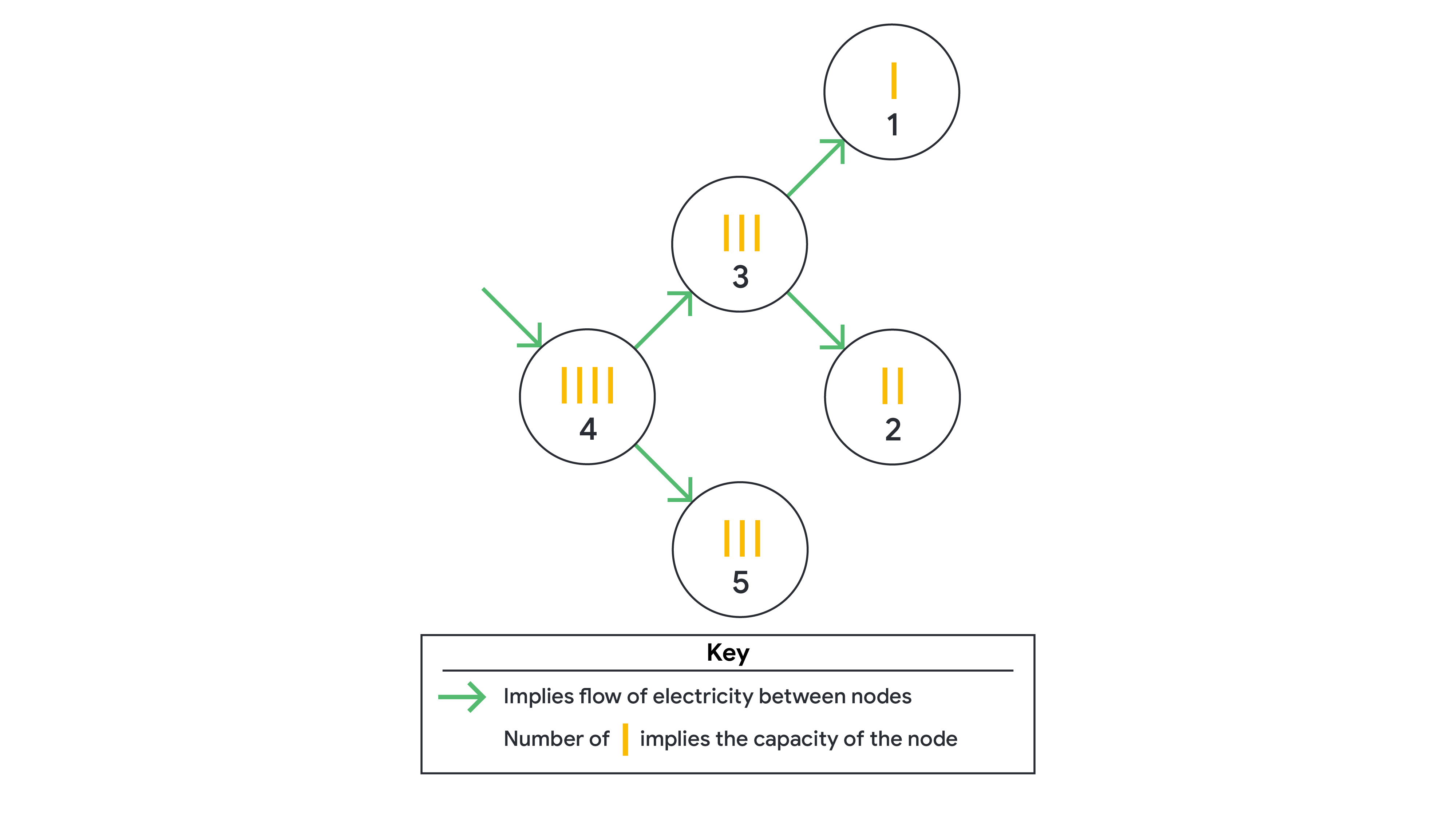
In Sample Case #1, the optimal solution is to provide electricity to the fourth junction. This
will transmit electricity to all the junctions eventually.
If the electricity is provided to the third junction, it
will transmit it to the first and second junction, but not to the fourth
junction. In that case, only three junctions can finally receive electricity.
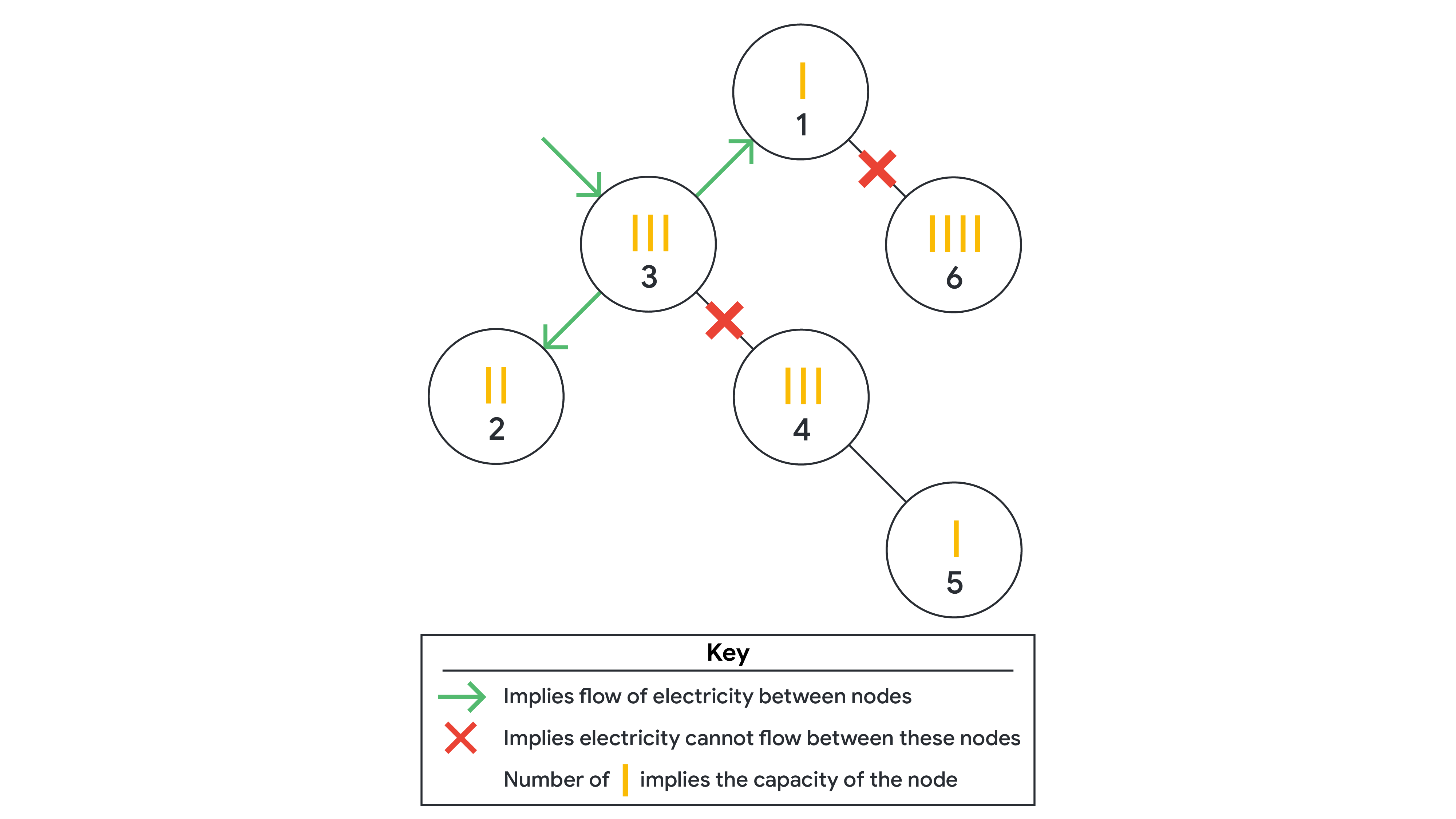
In Sample Case #2, the optimal solution is to provide electricity to the third junction.
This will transmit it to the first and second junctions.
Note that electricity will not be transmitted to the fourth junction,
since its capacity is not strictly less than that of the third junction.
If electricity is provided to the sixth junction, it will only be transmitted to
the first junction.
If electricity is provided to the fourth junction, it will only be transmitted to
the fifth junction.
D. Level Design
Problem
A permutation cycle in a permutation $$$C$$$ is a sequence of integers $$$(a_1, a_2, \dots, a_k)$$$ such that the following hold:
- $$$a_i \in C$$$ for all $$$i$$$, and are distinct.
- For each $$$i \in \{1, 2, \ldots, k-1\}$$$: $$$C[a_i] = a_{i+1}$$$, and $$$C[a_k] = a_1$$$.
A permutation cycle of length $$$k$$$ is called a $$$k$$$-cycle.
For example, the permutation $$$C = [4, 2, 1, 3]$$$ has two cycles: the $$$3$$$-cycle $$$(4, 3, 1)$$$, and the $$$1$$$-cycle $$$(2)$$$. $$$(4, 3, 1)$$$ is a cycle because $$$C[4] = 3$$$, $$$C[3] = 1$$$, and $$$C[1] = 4$$$.
Grace loves permutation cycles, so Charles decides to design an $$$\mathbf{N}$$$-level game to challenge her.
At the start of the game, the player is given an $$$\mathbf{N}$$$-length permutation $$$\mathbf{P}$$$ of integers from $$$1$$$ through $$$\mathbf{N}$$$. The levels in the game are numbered from $$$1$$$ to $$$\mathbf{N}$$$. At each level, the player starts with the given permutation, and is allowed to make modifications to it by swapping any two elements in it (multiple swaps allowed). To clear the $$$k$$$-th level in the game, the player is required to find the minimum number of swaps using which a $$$k$$$-cycle can be created in the permutation. The player can progress to the $$$(k+1)$$$-th level only after clearing the $$$k$$$-th level.
Grace finds the game a bit challenging, but wants to win at any cost. She needs your help! Formally, for each level $$$k$$$, you need to find the minimum number of swaps using which a $$$k$$$-cycle can be created in the permutation.
Input
The first line of the input gives the number of test cases, $$$\mathbf{T}$$$. $$$\mathbf{T}$$$ test cases follow.
The first line of each test case contains an integer $$$\mathbf{N}$$$: the length of the permutation.
The next line contains $$$\mathbf{N}$$$ integers $$$\mathbf{P_1}$$$, $$$\mathbf{P_2}$$$, $$$\dots$$$, $$$\mathbf{P_N}$$$, where the $$$i$$$-th
integer represents the $$$i$$$-th element in the permutation $$$\mathbf{P}$$$.
Output
For each test case, output one line containing Case #$$$x$$$: $$$S_1, S_2, \dots, S_N$$$,
where $$$x$$$ is the test case number (starting from 1), and $$$S_i$$$ is the solution for the
$$$i$$$-th level in the game, that is, the minimum number of swaps needed to create an
$$$i$$$-cycle in the permutation.
Limits
Time limit: 20 seconds.
Memory limit: 1 GB.
$$$1 \le \mathbf{T} \le 100$$$.
$$$1 \le \mathbf{P_i} \le \mathbf{N}$$$, for all $$$i$$$.
All $$$\mathbf{P_i}$$$ are distinct.
Test Set 1
$$$1 \le \mathbf{N} \le 10^3$$$.
Test Set 2
$$$1 \le \mathbf{N} \le 10^5$$$.
Sample
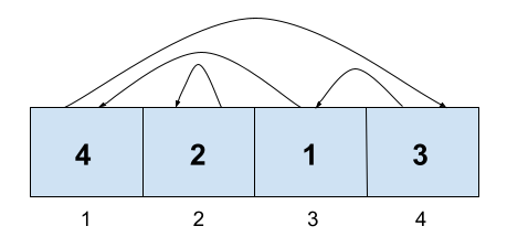
2
3
1 2 3
4
4 2 1 3
Case #1: 0 1 2
Case #2: 0 1 0 1
In Sample Case #1, there are three $$$1$$$-cycles in the given permutation. So, the first level can be cleared with zero swaps. To clear the second level, we can swap the first two elements to get the permutation $$$[2, 1, 3]$$$, which contains the $$$2$$$-cycle $$$(2, 1)$$$. To clear the third level, we can swap the first two elements, followed by the second and third elements to get the permutation $$$[2, 3, 1]$$$, which contains the $$$3$$$-cycle $$$(2, 3, 1)$$$.
In Sample Case #2, as explained earlier, the permutation has the $$$1$$$-cycle $$$(2)$$$. So, zero swaps are needed to clear the first level. To clear the second level, we can swap the last two elements to get the permutation $$$[4, 2, 3, 1]$$$, which contains the $$$2$$$-cycle $$$(4, 1)$$$. Since the permutation also has the $$$3$$$-cycle $$$(4, 3, 1)$$$, the third level can also be cleared using zero swaps. To clear the fourth level, we can swap the second and the fourth elements to get the permutation $$$[4, 3, 1, 2]$$$, which contains the $$$4$$$-cycle $$$(4, 2, 3, 1)$$$.
Analysis — A. Running in Circles
Test Set 1
Since Ada only runs in the clockwise direction, we can ignore the direction input altogether as Ada will always cross the starting line in the same direction she had last crossed it. Now, we can calculate the total distance run by Ada by calculating the sum:
This sum can be calculated while reading the input line-by-line and adding to $$$dist$$$, so we do not need to store the value of each $$$\mathbf{D_i}$$$. Then, we can calculate $$$\lfloor\frac{dist}{\mathbf{L}}\rfloor$$$, and obtain the number of laps the machine has counted.
Time and Space Complexity: This solution will run in $$$O(\mathbf{N})$$$ time and take up $$$O(1)$$$ extra space.
Test Set 2
Going through the input line-by-line, we calculate how much Ada has to run to be able to reach the starting line again (that is, the remaining distance to starting line, $$$R$$$) from the Ada's current position $$$pos$$$ ($$$pos = 0$$$ initially) before a run and in the current direction $$$\mathbf{C_i}$$$. We also keep track of the previous direction $$$prevdir$$$ she was running in when she last crossed the starting line.
$$$R$$$ can be calculated as follows:
- If $$$\mathbf{C_i}$$$ is clockwise, $$$R = (\mathbf{L} - pos) \bmod \mathbf{L}$$$
- If $$$\mathbf{C_i}$$$ is anticlockwise, $$$R = pos$$$
During each run (that is, for each line of input):
-
If $$$\mathbf{D_i} \lt R$$$, then we will just update her position
$$$pos$$$, as she can not reach the starting line.
- If $$$\mathbf{C_i}$$$ is clockwise, $$$pos = pos + \mathbf{D_i}$$$
- If $$$\mathbf{C_i}$$$ is anticlockwise, $$$pos = pos - \mathbf{D_i}$$$
After this update, we continue to the next run without updating $$$prevdir$$$ as Ada has not crossed the line this time.
-
On the other hand if $$$\mathbf{D_i} \ge R$$$, and if $$$R \gt 0$$$, we increase the number of laps by $$$1$$$ if $$$\mathbf{C_i}$$$ is the same as $$$prevdir$$$. However, if $$$R = 0$$$ (that is, Ada is exactly at the starting line), we do not perform this increment since Ada had already reached the starting line in the previous run, where it was counted as a lap by the machine (similarly for $$$R \lt 0$$$). Thus, we do not treat starting a run at the line as "crossing" the line, rather, we count a lap when Ada finishes at the line. With this logic, the case where Ada changes her direction on the line itself will also not be counted as a lap.
We then increase the number of laps by the value $$$\lfloor\frac{\mathbf{D_i} - R}{\mathbf{L}}\rfloor$$$ to take care of cases where multiple laps are made in a single run (this will also handle the above case, where Ada just reaches the starting line after a run). As these laps are counted from the starting line, $$$prevdir$$$ does not matter in this calculation. Then, we update Ada's current position:
- If $$$\mathbf{C_i}$$$ is clockwise, $$$pos = (\mathbf{D_i} - R) \bmod \mathbf{L}$$$
- If $$$\mathbf{C_i}$$$ is anticlockwise, $$$pos = \mathbf{L} - ((\mathbf{D_i} - R) \bmod \mathbf{L})$$$
After the above process, we update $$$prevdir$$$ to $$$\mathbf{C_i}$$$ and continue.
Finally, return the number of laps counted.
Time and Space Complexity: This solution also runs in $$$O(\mathbf{N})$$$ time, and takes up $$$O(1)$$$ extra space.
Analysis — B. Magical Well Of Lilies
Test Set 1
For the small test set, a simple backtracking algorithm is sufficiently fast. In each recursive call, we need to keep track of the number of lilies remaining in the well, the current state of well's memory, and the number of coins we have tossed so far. In each recursive step, we have at most three choices:
- Toss one coin for another lily;
- Toss two coins for as many lilies as last noted by the well;
- Toss six coins ($$$4+2$$$) for the well to remember the current state of the basket and then toss as many lilies.
Of course, we would consider an operation only if the well has that many lilies, for it would be a waste of coins otherwise. If the number of lilies left in the well becomes $$$0$$$ at any time of the recursion, we update the minimum number of coins, if necessary, and return immediately from the recursion.
Since we have at most three choices at each recursion level, the time complexity of this exhaustive search might seem like a prohibitive $$$O(3^\mathbf{L})$$$, however, the algorithm is much faster in practice for two reasons. First, not all three choices are available at each recursion level. And second, the maximal recursion depth of $$$\mathbf{L}$$$ is possible only if we pick up the lilies one by one. In other words, the average recursion depth is much smaller than $$$\mathbf{L}$$$. For example, the algorithm needs just $$$5060$$$ recursive calls for $$$\mathbf{L}=20$$$.
Test Set 2
For the large test set, the exhaustive search is obviously too slow as the number of recursive calls for $$$\mathbf{L}=50$$$ is already $$$7,821,316,841$$$. Fortunately, dynamic programming comes to rescue here.
But first, let us make one useful observation. Namely, we can always rearrange some operations such that a two coin operation never follows a one coin operation. If it does, we can always swap the two operations without affecting the net effect of the whole sequence of operations.
Now let us turn to our dynamic programming recurrence. Let $$$DP[i]$$$ be the minimum number of coins needed to fetch $$$i$$$ lilies from the well. We have $$$DP[0]=0$$$ and $$$DP[1]=1$$$. For $$$i > 1$$$, there are two possible ways of arriving at $$$i$$$ lilies — we either collect $$$i - 1$$$ lilies first and then use a one coin operation to get another lily, or the last operation must have been a two coin operation. The latter means that we had asked the well to remember the state of our basket at $$$k$$$ lilies (where $$$k$$$ is a divisor of $$$i$$$) and then applied $$$\frac{i}{k}-1$$$ two coin operations. Formally, $$$DP[i]=\min(DP[i - 1] + 1, \min\limits_{k|i}\{DP[k]+4+2(\frac{i}{k}-1)\})$$$.
In practice, instead of calculating each $$$DP[i]$$$ directly using the formula above and iterating over the divisors of $$$i$$$, we inverse the process as follows:
At the beginning we can say that all values of $$$DP$$$ except for $$$0$$$ and $$$1$$$ are equal to infinity. Now let us iterate through all $$$i$$$ from $$$2$$$ to $$$\mathbf{N}$$$. One option to use one coin and get from $$$i-1$$$ lilies to $$$i$$$ lilies, so we can say that $$$DP[i] = min(DP[i], DP[i-1]+1)$$$. Now when we already have $$$i$$$ lilies, we can also use four coins to remember the state of our basket and then later get $$$j \cdot i$$$ lilies from the well. So we should update $$$DP$$$ for all multiples of $$$i$$$: $$$ DP[j \cdot i] = min(DP[j \cdot i], DP[i] + 4 + 2 \cdot (j-1)) $$$ for $$$i < j \cdot i \leq \mathbf{N}$$$.
As for the time complexity of the algorithm, for each index $$$k$$$, there are $$$O(\frac{\mathbf{L}}{k})$$$ multiples to be updated, which leads to $$$O(\mathbf{L}(1+\frac{1}{2}+\frac{1}{3}+\ldots+\frac{1}{\mathbf{L}}))$$$ updates. The factor $$$1+\frac{1}{2}+\frac{1}{3}+\ldots+\frac{1}{\mathbf{L}}$$$ is the $$$\mathbf{L}$$$-th harmonic number, which is $$$O(\log \mathbf{L})$$$, therefore, the overall time complexity of the algorithm is $$$O(\mathbf{L} \log \mathbf{L})$$$.
As a final note, we can precompute the $$$DP$$$ table in advance, and then answer each test case in constant time.
Analysis — C. Electricity
Test Set 1
For this test set, we can simulate providing electricity to each junction, one junction at a time. For each of these $$$\mathbf{N}$$$ simulations, we compute how many junctions will end up receiving electricity after the initial junction is powered, and our answer is the maximum of these $$$\mathbf{N}$$$ simulation results. Each simulation can be accompolished with depth-first search (DFS); we start our DFS at the junction we are directly providing power to. In each step of our DFS, we iterate over the current junction's neighbors, and recurse into the neighbor if its capacity is strictly less than the current junction's capacity. Because the capacity must be strictly decreasing, we are guaranteed to never go in a cycle or visit a junction more than once. The DFS time complexity is therefore bounded by the total number of edges, making it take $$$O(\mathbf{N})$$$ time; with $$$\mathbf{N}$$$ simulations, this gives us an $$$O(\mathbf{N}^2)$$$ time solution, which is sufficient for this test set.
Test Set 2
We can improve our DFS-based solution from test set 1 to be fast enough for this test set by removing the redundancy among the $$$\mathbf{N}$$$ DFS invocations and consolidating the computation into an $$$O(\mathbf{N})$$$ solution. To give an example of the computational redundancy from our test set 1 solution that we aim to remove, suppose $$$v_1$$$ and $$$v_2$$$ are directly connected junctions, with $$$v_1$$$ having the greater capacity. Simulating providing electricity to $$$v_1$$$ will also lead to simulating providing electricity to $$$v_2$$$ due to the edge between them, but we will also simulate directly providing electricity to $$$v_2$$$, duplicating our work. We can remove this duplication by treating this as a dynamic programming problem and memoizing our work.
Our solution works similarly to before, where for each junction $$$v$$$ we perform a DFS to compute how many junctions would be powered if we provided electricity to $$$v$$$. However, we memoize this DFS; when the DFS is called on a junction $$$v$$$, we first check if $$$v$$$ is in our memoization table and return the result if it's present. Otherwise, we recurse and perform DFS as usual, but store the result in the memoization table before returning the result. This memoization implies that among our $$$\mathbf{N}$$$ DFS calls, an edge will never be traversed twice, because after the first traversal, the result will be memoized, making further traversals unnecessary. This implies our $$$\mathbf{N}$$$ DFS calls will take in total $$$O(\mathbf{N})$$$ time, making this approach sufficiently fast for the large test set.
Analysis — D. Level Design
We have been given a permutation $$$\mathbf{P}$$$ of length $$$\mathbf{N}$$$ and are asked to find minimum swaps required to form at least one permutation cycle of length $$$K$$$, for all $$$1 \leq K \leq \mathbf{N}$$$. Here are a few steps required to solve this problem.
- Step 1: Find the existing permutation cycles.
- Step 2: Analyze the effect of a swap in the permutation.
- Type 1: Swap within the same cycle, the cycle will be broken into two smaller cycles.
- Type 2: Swap two elements from different cycles, both the cycles will end up merging. The length of the new cycle will be the sum of lengths of two cycles merged.
- Step 3: Optimal merging for each cycle length.
Considering permutation
cycle as a graph, perform DFS from each unvisited node and keep traversing till we get a visited node. Maintain the cycle length for each DFS.
At the end of this we have an array representing cycle lengths of the permutation cycles. Alternative approach is to use DSU to find all cycles and respective lengths.
Let us name the cycle size array as $$$\text{cycle_sizes}$$$.
Two types of swaps are possible:
Now we know the existing cycle lengths and the effect of a swap, we need to find the optimal strategy to form a cycle of length $$$K$$$ in the minimum number of swaps.
Now the problem essentially boils down to optimally selecting the cycles to merge/break to form a cycle of length $$$K$$$.
There are two potential strategies:
1) We can sort the cycle lengths in descending order by length and then merge the cycles starting from the maximum one till we get a final cycle of length
$$$ > K$$$ and then use one more swap to turn that into exactly $$$K$$$. The number of steps required here is an upper bound on the optimal number of swaps and the lower bound will be at least one less than the
upper bound (forming cycle of exact length $$$K$$$). Time complexity of greedy approach is $$$O(\mathbf{N})$$$ since sorting the permutation cycles itself will take $$$O(\mathbf{N})$$$ using Counting sort.
2) We can apply dynamic programming to optimally find minimum number of cycles required to form a cycle of size exactly $$$K$$$.
The optimal strategy is to choose the minimum of the two strategies.
Test Set 1
For each of the cycles we do have the option either to include it in the optimal set of cycles to be merged or leave it. This problem is now very similar to the
knapsack problem.
Let $$$dp(i, j) $$$ be the minimum number of swaps required to form a cycle of length j using cycles from indices $$$(1, i)$$$.
$$$dp(i, j) = \min(dp(i - 1, j), 1 + dp(i - 1, j - \text{cycle_sizes(i)})) $$$
$$$ S = \text{cycle_sizes.size()}$$$.
We need to populate the $$$dp$$$ table with the above mentioned recurrence relation. $$$dp(S, K)$$$ is the answer from the knapsack approach and
$$$\min(1 + dp(S, t)) $$$ for all $$$K+ 1 \leq t \leq \mathbf{N}$$$ is the answer from greedy approach. Final answer will be minimum of both the
values.
Time complexity will be $$$O(\mathbf{N}^2)$$$ to populate the $$$dp$$$ table.
Test Set 2
Let $$$X$$$ be the number of length wise distinct cycles, minimum number of nodes required to form all the $$$X$$$ cycles
is $$$\sum_{i = 1}^{X}i$$$. As per the constraints, $$$\sum_{i = 1}^{X}i \leq \mathbf{N}$$$.
Hence there will be $$$O(\sqrt{\mathbf{N}})$$$ number of length wise distinct cycles. Using this fact we can speed up our knapsack-based solution from test set 1.
Let us name the distinct cycle size array as $$$\text{distinct_cycle_sizes}$$$ and corresponding occurrences as $$$\text{cnt}$$$.
Let $$$dp(i, j) $$$ be the minimum number of swaps required to form a cycle of length j using cycles from indices $$$ (1, i)$$$ where $$$1 \leq i \leq \text{distinct_cycle_sizes.size()}$$$.
Hence, in order to calculate $$$dp(i, j)$$$ (where i is the index of the current value $$$x$$$ being processed and $$$j$$$ is the cost), we only need these states
$$$dp(i - 1, j - x), dp(i - 1, j - 2 \times x), \dots, dp(i - 1, j - cnt(i) \times x)$$$.
For each distinct cycle size, store its number of occurrences and then the idea to process
$$$v$$$(occurrences of each cycle) items of value $$$x$$$ is to treat the problem as a
sliding window minimum problem.
Hence, the recurrence becomes $$$ dp(i, j) = \min(v + dp(i - 1, j - v \times \text{distinct_cycle_sizes}[i]), v \in [0, cnt(i)]$$$
Then, if we consider the values $$$j \mod k$$$, you will notice that for a fixed remainder it just becomes a range min query on a 'sliding window' interval (namely, the left bound of the interval may only move to the right each query), which can be computed in amortized constant time using a monotonic deque.
So, now for each $$$i \in [1, \mathbf{N}]$$$, the optimal answer $$$= \min(dp(\text{items_count}, i), dp(\text{items_count}, j) + 1)$$$ where $$$j > i$$$.
Complexity will be $$$O(\mathbf{N}\sqrt{\mathbf{N}})$$$ to populate the $$$dp$$$ table.
Sample Code (C++)
const int inf = 1e9;
void knapsack(vector<int> distinct_cycle_sizes, vector<vector<int>> dp, vector<int> cnt, int n) {
  dp[0][0] = 0;
  for(int i = 1; i <= (int)distinct_cycle_sizes.size(); ++i) {
    int cs = distinct_cycle_sizes[i - 1];
    dp[i][0] = 0;
    // Using standard sliding window approach.
    for(int j = 0; j < cs; ++j) {
      deque<int> dq;
      for(int l = j; l <= n; l += cs) {
        dp[i][l] = min(dp[i][l], dp[i - 1][l]);
        int opt = inf, x = -1;
        if(l and !dq.empty()) {
          opt = dp[i - 1][dq.front()] + (l - dq.front()) / cs;
          x = dq.front();
        } else if(!l) {
          opt = 0;
        }
        dp[i][l] = min(dp[i][l], opt);
        while(!dq.empty() and dq.front() <= l - cnt[cs] * cs) {
          dq.pop_front();
        }
        while(!dq.empty() and dp[i - 1][l] <= dp[i - 1][dq.back()]) {
          dq.pop_back();
        }
        dq.push_back(l);
      }
    }
  }
  vector<int> fans(n + 1);
  int best_right = inf, items_count = distinct_cycle_sizes.size();
  for(int i = n; i >= 1; --i) {
    // best_right + 1 accounts for greedy.
    fans[i] = min(dp[items_count][i], best_right + 1);
    best_right = min(best_right, fans[i]);
  }
  for(int i = 1; i <= n; ++i) {
    cout << fans[i] - 1 << " ";
  }
  return;
}