Google Kick Start Archive — Round F 2022 problems
Overview
Thank you for participating in Kick Start 2022 Round F!
Cast
Sort the Fabrics: Written by Ryan Moore and prepared by Shubham Avasthi.
Water Container System: Written by Anurag Singh and prepared by Chu-ling Ko.
Story of Seasons: Written by Chu-ling Ko and prepared by Chun-nien Chan.
Scheduling a Meeting: Written by Adilet Zhaxybay and prepared by Viktoriia Kovalova.
Solutions, other problem preparation, reviews and contest monitoring by Adilet Zhaxybay, Aman Singh, Anurag Singh, Anushi Maheshwari, Ashutosh Bang, Bakuri Tsutskhashvili, Bartosz Kostka, Bohdan Pryshchenko, Brijesh Panara, Chu-ling Ko, Chun-nien Chan, Cristhian Bonilha, Deepanshu Aggarwal, Diksha Saxena, Gagan Kumar, Hana Joo, Jackie Cheung, Jimmy Dang, Krists Boitmanis, Lizzie Sapiro Santor, Lucas Maciel, Pratibha Jagnere, Priyam Khandelwal, Rahul Goswami, Rohan Garg, Ryan Moore, Sachin Yadav, Sadia Atique, Sanyam Garg, Shubham Avasthi, Sourabh Pukale, Surya Upadrasta, Swapnil Gupta, Tarun Khullar, Teja Vardhan Reddy Dasannagari, Umang Goel, Viktoriia Kovalova, Vinamra Bathwal, Vinay Khilwani, Vishal Som, Wei Zhou, Yang Zheng.
Analysis authors:
- Sort the Fabrics: Sadia Atique
- Water Container System: Krists Boitmanis
- Story of Seasons: Chu-ling Ko
- Scheduling a Meeting: Adilet Zhaxybay
A. Sort the Fabrics
Problem
A fabric is represented by three properties:
- Color ($$$\mathbf{C}$$$), a string consisting of lowercase letters of the English alphabet, representing the color of the fabric.
- Durability ($$$\mathbf{D}$$$), an integer representing the durability of the fabric.
- Unique identifier ($$$\mathbf{U}$$$), an integer representing the ID of the fabric.
Ada and Charles work at the Kick Start fabric factory. Each day they receive $$$\mathbf{N}$$$ fabrics, and one of them has to sort it. They sort it using the following criteria:
- Ada sorts in lexicographically increasing order by color ($$$\mathbf{C}$$$).
- Charles sorts in ascending order by durability ($$$\mathbf{D}$$$).
- They break ties by sorting in ascending order by the unique identifier ($$$\mathbf{U}$$$).
Given $$$\mathbf{N}$$$ fabrics, count the number of fabrics which end up in the same position regardless of whether Ada or Charles sort them.
Input
The first line of the input gives the number of test cases, $$$\mathbf{T}$$$. $$$\mathbf{T}$$$ test cases follow.
Each test case begins with one line consisting of an integer $$$\mathbf{N}$$$ denoting the number of fabrics. Then
$$$\mathbf{N}$$$ lines follow, each line with a string $$$\mathbf{C_i}$$$, an integer $$$\mathbf{D_i}$$$, and an integer $$$\mathbf{U_i}$$$: the color, the
durability and the unique identifier of the $$$i$$$-th fabric respectively.
Output
For each test case, output one line containing Case #$$$x$$$: $$$y$$$,
where $$$x$$$ is the test case number (starting from 1) and $$$y$$$ is the number of fabrics which
end up in the same position regardless of whether a worker sorts them by color or by durability.
Limits
Time limit: 20 seconds.
Memory limit: 1 GB.
$$$1 \le \mathbf{T} \le 100$$$.
$$$1 \le$$$ length of string $$$\mathbf{C_i}$$$ $$$\le 10$$$.
String $$$\mathbf{C_i}$$$ consists of only lowercase letters of the English alphabet.
No two fabrics have same $$$\mathbf{U_i}$$$.
Test Set 1
$$$1 \le \mathbf{N} \le 2$$$.
$$$1 \le \mathbf{D_i} \le 2$$$.
$$$1 \le \mathbf{U_i} \le 2$$$.
Test Set 2
$$$1 \le \mathbf{N} \le 10^3$$$.
$$$1 \le \mathbf{D_i} \le 10^2$$$.
$$$1 \le \mathbf{U_i} \le 10^3$$$.
Sample
Note: there are additional samples that are not run on submissions down below.3 2 blue 2 1 yellow 1 2 2 blue 2 1 brown 2 2 1 red 1 1
Case #1: 0
Case #2: 2
Case #3: 1
In Sample Case #1, when sorted by color, the order of fabrics represented by the unique identifier is $$$1$$$ and $$$2$$$. When sorted by durability, the order of fabrics is $$$2$$$ and $$$1$$$. Therefore, $$$0$$$ fabrics have the same position when sorted by color or durability.
In Sample Case #2, when sorted by color, the order of fabrics represented by the unique identifier is $$$1$$$ and $$$2$$$. When sorted by durability, the order of fabrics is also $$$1$$$ and $$$2$$$. Therefore, $$$2$$$ fabrics have the same position. Notice that both fabrics have the same durability, so when Charles sorts them he decides that fabric $$$1$$$ comes first because it has a smaller identifier.
In Sample Case #3, since there is only $$$1$$$ fabric, the position remains the same whether the fabrics are sorted by color or durability.
Additional Sample - Test Set 2
The following additional sample fits the limits of Test Set 2. It will not be run against your submitted solutions.1 5 blue 1 2 green 1 4 orange 2 5 red 3 6 yellow 3 7
Case #1: 5
In Sample Case #1, the order is the same for both when sorted by color or durability. So the answer is $$$5$$$.
B. Water Container System
Problem
There is a water container system with $$$\mathbf{N}$$$ identical containers, which can be represented as a tree, where each container is a vertex. The containers are connected to each other with $$$\mathbf{N}-1$$$ bidirectional pipes. Two containers connected to each other are always placed on adjacent levels. Formally, if two containers $$$a$$$ and $$$b$$$ are connected to each other, then $$$|level_a - level_b | = 1$$$. Container $$$1$$$ is placed at the bottommost level. Each container is connected to exactly one container on the level below (the only exception is container $$$1$$$, which has no connections below it), but can be connected to zero or more containers on the level above. The maximum capacity of each container is $$$1$$$ liter, and initially all the containers are empty. Assume that the pipe has a capacity of $$$0$$$ liters. In other words, they do not store any water, but only allow water to pass through them in any direction.
Consider the following diagram which is an example of a water container system:
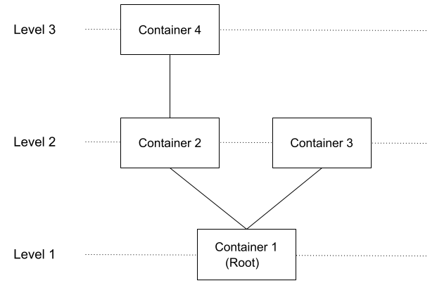
The first level of the system consists of a single container, container $$$1$$$ (root). Container $$$1$$$ is connected to container $$$2$$$ and container $$$3$$$, which are present in the above level, level $$$2$$$. Container $$$2$$$ is also connected to container $$$4$$$, which is present at level $$$3$$$.
You are given $$$\mathbf{Q}$$$ queries. Each query contains a single integer $$$i$$$ which represents a container. For each query, add an additional $$$1$$$ liter of water in container $$$i$$$.
The following diagram illustrates the flow of the water in the system in different conditions:
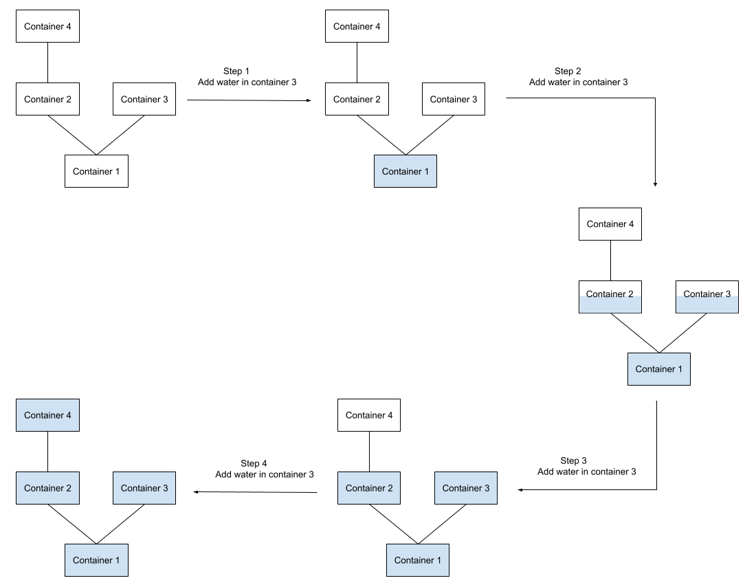
In step $$$1$$$, after adding $$$1$$$ liter of water in container $$$3$$$, the
water flows downward because the water containers at the lower level are still
empty.
In step $$$2$$$, after adding $$$1$$$ liter of water in container $$$3$$$, the
water flows downward, but as the container $$$1$$$ is already filled
completely, the water is distributed evenly between water containers $$$2$$$
and $$$3$$$.
In step $$$3$$$, after adding $$$1$$$ liter of water in container $$$3$$$, the
water containers $$$2$$$ and $$$3$$$ are completely filled.
In step $$$4$$$, after adding $$$1$$$ liter of water in container $$$3$$$, the
water is pushed up to water container $$$4$$$, which is then completely
filled.
As illustrated in the example above, containers at the same level will have the same amount of water. Find the number of water containers that are completely filled after processing all the queries.
Input
The first line of the input gives the number of test cases, $$$\mathbf{T}$$$. $$$\mathbf{T}$$$ test
cases follow.
The first line of each test case contains the two integers $$$\mathbf{N}$$$ and $$$\mathbf{Q}$$$, where
$$$\mathbf{N}$$$ is the number of containers and $$$\mathbf{Q}$$$ is the number of queries.
The next $$$\mathbf{N}-1$$$ lines contain two integers $$$i$$$ and $$$j$$$ ($$$1 \le
i, j \le \mathbf{N}$$$, and $$$i ≠ j$$$) meaning that the $$$i$$$-th water
container is connected to the $$$j$$$-th water container.
Each of the next $$$\mathbf{Q}$$$ lines contain a single integer $$$i$$$ ($$$1 \le i \le
\mathbf{N}$$$) that represents the container to which $$$1$$$ liter of water should
be added.
Output
For each test case, output one line containing
Case #$$$x$$$: $$$y$$$, where $$$x$$$ is the test case number
(starting from 1) and $$$y$$$ is the number of water containers that are
completely filled after processing all the queries.
Limits
Memory limit: 1 GB.
$$$1 \le \mathbf{T} \le 100$$$.
$$$1 \le \mathbf{Q} \le \mathbf{N}$$$.
It is guaranteed that the given water container system is a tree.
Test Set 1
Time limit: 20 seconds.
$$$1 \le \mathbf{N} \le 65535$$$.
The water container system is a
perfect binary tree.
Test Set 2
Time limit: 60 seconds.
$$$1 \le \mathbf{N} \le 10^4$$$.
Sample
Note: there are additional samples that are not run on submissions down below.2 1 1 1 3 2 1 2 1 3 1 2
Case #1: 1
Case #2: 1
In Sample Case #1, there is $$$\mathbf{N} = 1$$$ water container. The number of completely filled water containers after adding $$$1$$$ liter of water in container $$$1$$$ is $$$1$$$.
In Sample Case #2, there are $$$\mathbf{N} = 3$$$ water containers. The number of completely filled water containers after processing all the queries is $$$1$$$.
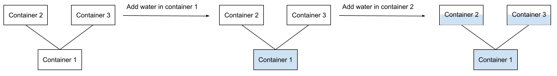
After adding $$$1$$$ liter of water in container $$$1$$$: container $$$1$$$
is completely filled, and the remaining containers are empty.
After adding $$$1$$$ liter of water in container $$$2$$$: container $$$1$$$
is completely filled, and containers $$$2$$$ and $$$3$$$ are partially
filled.
Additional Sample - Test Set 2
The following additional sample fits the limits of Test Set 2. It will not be run against your submitted solutions.2 4 4 1 2 1 3 2 4 3 3 3 3 5 2 1 2 5 3 3 1 2 4 4 5
Case #1: 4
Case #2: 1
In Sample Case #1, there are $$$\mathbf{N} = 4$$$ water containers. The number of completely filled water containers after processing all the queries is $$$4$$$, which is already explained in the problem statement.
In Sample Case #2, there are $$$\mathbf{N} = 5$$$ water containers. The number of completely filled water containers after processing all the queries is $$$1$$$.
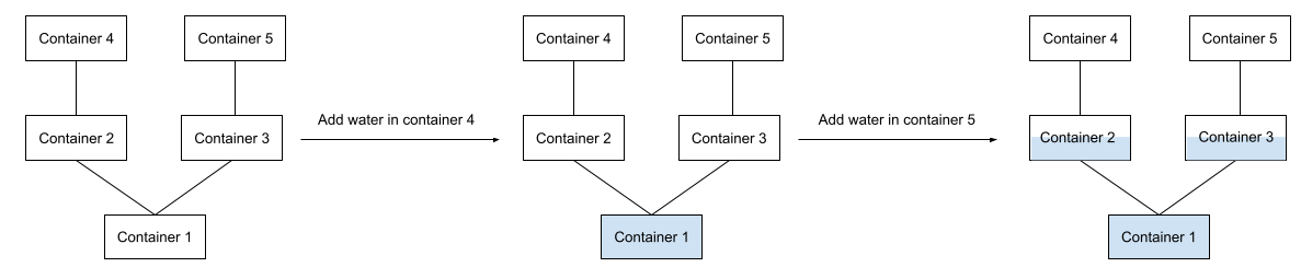
After adding $$$1$$$ liter of water in container $$$4$$$: container $$$1$$$
is completely filled, and the remaining containers are empty.
After adding $$$1$$$ liter of water in container $$$5$$$: container $$$1$$$
is completely filled, containers $$$2$$$ and $$$3$$$ are partially filled,
and the remaining containers are empty.
C. Story of Seasons
Problem
You are a super farmer with some vegetable seeds and an infinitely large farm. In fact, not only are you a farmer, but you are also secretly a super programmer! As a super programmer, you hope to maximize the profit of your farming using your programming skills.
Since your daily energy is limited, you can plant at most $$$\mathbf{X}$$$ seeds each day. In the beginning, you have $$$\mathbf{N}$$$ kinds of vegetable seeds. The number of seeds of the $$$i$$$-th kind of vegetable is $$$\mathbf{Q_i}$$$, and each seed of this kind needs $$$\mathbf{L_i}$$$ days to mature from the day it is planted. Once it matures, you can sell it for $$$\mathbf{V_i}$$$ dollars. Assume that no energy or time is required for harvesting and selling vegetables. Also, your farm is infinitely large so the growing vegetables do not crowd out each other.
Notice that although the area of your farm is infinite, the number of days that you can plant seeds is limited. The warm season only lasts $$$\mathbf{D}$$$ days, and after that, the harsh winter comes. Any vegetable that has not matured yet will die immediately and cannot be turned into profit. The remaining seeds that were not planted cannot be turned into profit either.
As a super farmer and a super programmer, you want to come up with a perfect planting plan that will maximize your profit. Find the total amount of profit you will earn.
Input
The first line of the input gives the number of test cases, $$$\mathbf{T}$$$. $$$\mathbf{T}$$$ test cases follow.
The first line of each test case contains three integers $$$\mathbf{D}$$$, $$$\mathbf{N}$$$, and $$$\mathbf{X}$$$: the number of days of
the warm season, the number of kinds of vegetable seeds you have to start with, and the maximum number
of seeds you can plant each day, respectively.
The next $$$\mathbf{N}$$$ lines describe the seeds. The $$$i$$$-th
line contains three integers $$$\mathbf{Q_i}$$$, $$$\mathbf{L_i}$$$, and $$$\mathbf{V_i}$$$: the quantity of this kind of seed, the
number of days it needs to mature, and the value of each matured plant, respectively.
Output
For each test case, output one line containing Case #$$$x$$$: $$$y$$$,
where $$$x$$$ is the test case number (starting from 1) and $$$y$$$ is the maximum amount of money
you can earn by optimizing your farming plan.
Limits
Memory limit: 1 GB.
$$$1 \le \mathbf{T} \le 100$$$.
$$$1 \le \mathbf{V_i} \le 10^6$$$, for all $$$i$$$.
$$$1 \le \mathbf{L_i} \le \mathbf{D}$$$, for all $$$i$$$.
Test Set 1
Time limit: 20 seconds.
$$$2 \le \mathbf{D} \le 1000$$$.
$$$1 \le \mathbf{N} \le 15$$$.
$$$\mathbf{X} = 1$$$.
$$$\mathbf{Q_i} = 1$$$, for all $$$i$$$.
Test Set 2
Time limit: 60 seconds.
$$$2 \le \mathbf{D} \le 10^5$$$.
$$$1 \le \mathbf{N} \le 10^5$$$.
$$$1 \le \mathbf{X} \le 10^9$$$.
$$$1 \le \mathbf{Q_i} \le 10^6$$$, for all $$$i$$$.
Test Set 3
Time limit: 60 seconds.
$$$2 \le \mathbf{D} \le 10^{12}$$$.
$$$1 \le \mathbf{N} \le 10^5$$$.
$$$1 \le \mathbf{X} \le 10^9$$$.
$$$1 \le \mathbf{Q_i} \le 10^6$$$, for all $$$i$$$.
$$$\mathbf{D} \times \mathbf{X} \le 10^{18}$$$.
Sample
Note: there are additional samples that are not run on submissions down below.2 5 4 1 1 2 3 1 3 10 1 4 5 1 2 2 5 1 1 1 1 1
Case #1: 18
Case #2: 1
In Sample Case #1, there are $$$\mathbf{D} = 5$$$ days, $$$\mathbf{N} = 4$$$ kinds of vegetables and you can plant at most $$$\mathbf{X} = 1$$$ seed each day. Supposing the $$$4$$$ kinds of vegetables are spinach, pumpkin, carrot and cabbage, we have that
- Spinach needs $$$2$$$ days to grow, each matured one is worth $$$3$$$ dollars, and you start with $$$1$$$ spinach seed.
- Pumpkin needs $$$3$$$ days to grow, each matured one is worth $$$10$$$ dollars, and you start with $$$1$$$ pumpkin seed.
- Carrot needs $$$4$$$ days to grow, each matured one is worth $$$5$$$ dollars, and you start with $$$1$$$ carrot seed.
- Cabbage needs $$$2$$$ days to grow, each matured one is worth $$$2$$$ dollars, and you start with $$$1$$$ cabbage seed.
The maximum profit you can make is $$$18$$$ dollars. One of the schedules you can use is:
- Day 1: plant $$$1$$$ carrot
- Day 2: plant $$$1$$$ pumpkin
- Day 3: plant $$$1$$$ spinach
- Day 4: plant $$$1$$$ cabbage
- Day 5: do nothing
And with this schedule, the vegetables will mature and turn into profit as following days:
- Day 1: nothing harvested
- Day 2: nothing harvested
- Day 3: nothing harvested
- Day 4: nothing harvested
- Day 5: $$$1$$$ spinach, $$$1$$$ pumpkin and $$$1$$$ carrot harvested, you earn $$$18$$$ dollars
Note that the cabbage is supposed to mature on day $$$6$$$, but it will actually die because of the winter.
Additional Sample - Test Set 2
The following additional sample fits the limits of Test Set 2. It will not be run against your submitted solutions.1 5 3 4 5 2 3 2 3 10 2 4 5
Case #1: 45
In Additional Sample Case #1, there are $$$\mathbf{D} = 5$$$ days, $$$\mathbf{N} = 3$$$ kinds of vegetables and you can plant at most $$$\mathbf{X} = 4$$$ seeds each day. Supposing the $$$3$$$ kinds of vegetables are spinach, pumpkin and carrot, we have that
- Spinach needs $$$2$$$ days to grow, each matured one is worth $$$3$$$ dollars, and you start with $$$5$$$ spinach seeds.
- Pumpkin needs $$$3$$$ days to grow, each matured one is worth $$$10$$$ dollars, and you start with $$$2$$$ pumpkin seeds.
- Carrot needs $$$4$$$ days to grow, each matured one is worth $$$5$$$ dollars, and you start with $$$2$$$ carrot seeds.
The maximum profit you can make is $$$45$$$ dollars. One of the schedules you can use is:
- Day 1: plant $$$1$$$ pumpkin, $$$2$$$ carrots and $$$1$$$ spinach
- Day 2: plant $$$2$$$ spinach and $$$1$$$ pumpkin
- Day 3: plant $$$2$$$ spinach
- Day 4: do nothing
- Day 5: do nothing
And with this schedule, the vegetables will mature and turn into profit as following days:
- Day 1: nothing harvested
- Day 2: nothing harvested
- Day 3: $$$1$$$ spinach harvested, you earn $$$3$$$ dollars
- Day 4: $$$2$$$ spinach and $$$1$$$ pumpkin harvested, you earn $$$16$$$ dollars
- Day 5: $$$2$$$ spinach, $$$1$$$ pumpkin and $$$2$$$ carrots harvested, you earn $$$26$$$ dollars
D. Scheduling a Meeting
Problem
Scheduling meetings at Google is not an easy task. Even with the help of Google Calendar, Ada has a lot of difficulty with it!
Ada works as a Software Engineer at Google, and needs to get approval for her new project. In order to get an approval, she needs to meet with at least $$$\mathbf{K}$$$ of $$$\mathbf{N}$$$ Tech Leads.
Ada has access to the calendars of all $$$\mathbf{N}$$$ Tech Leads. For each Tech Lead, Ada can see all their scheduled meetings. The timeline in this problem can be viewed as $$$\mathbf{D}$$$ consecutive hours, and all meetings are in $$$[0, \mathbf{D}]$$$ hours range, with both ends being integer numbers. Scheduled meetings, even for the same person, can overlap (people are notorious for this at Google!).
Ada needs to schedule an $$$\mathbf{X}$$$-hour-long meeting in the interval of $$$[0, \mathbf{D}]$$$ hours, with both ends being integer numbers as well. At least $$$\mathbf{K}$$$ of $$$\mathbf{N}$$$ Tech Leads should be present for the whole meeting, that is their calendar should be completely free for the entire meeting duration.
Unfortunately, it might be the case that it is already impossible to find a slot to schedule such an $$$\mathbf{X}$$$-hour-long meeting. In that case, Ada will need to persuade some Tech Leads to cancel their existing meetings.
What is the minimum number of scheduled meetings that need to be canceled so that Ada can meet with at least $$$\mathbf{K}$$$ Tech Leads?
Input
The first line of the input gives the number of test cases, $$$\mathbf{T}$$$. $$$\mathbf{T}$$$ test cases follow.
The first line of each test case contains four integers $$$\mathbf{N}$$$, $$$\mathbf{K}$$$, $$$\mathbf{X}$$$, $$$\mathbf{D}$$$. $$$\mathbf{N}$$$ represents the number of Tech Leads, $$$\mathbf{K}$$$ is the minimum number of Tech Leads Ada needs to meet, $$$\mathbf{X}$$$ is the length of the meeting that needs to be set up, and $$$\mathbf{D}$$$ is the upper bound of the $$$[0, \mathbf{D}]$$$ hour range representing the timeline of the problem — no meeting can end after $$$\mathbf{D}$$$.
The second line of each test case contains an integer $$$\mathbf{M}$$$, representing the number of scheduled meetings.
$$$\mathbf{M}$$$ lines follow. The $$$i$$$-th of these contains three integer numbers $$$\mathbf{P_i}$$$, $$$\mathbf{L_i}$$$, and $$$\mathbf{R_i}$$$. These numbers represent that a Tech Lead $$$\mathbf{P_i}$$$ has a scheduled meeting between the hours $$$\mathbf{L_i}$$$ and $$$\mathbf{R_i}$$$, not including the endpoints (that is, the meeting can be seen as an $$$(\mathbf{L_i}, \mathbf{R_i})$$$ interval).
Note that all $$$\mathbf{M}$$$ meetings in the test case are independent, even if some of them have the same starting and ending time.
Output
For each test case, output one line containing
Case #$$$x$$$: $$$y$$$, where $$$x$$$ is the test case number
(starting from 1) and $$$y$$$ is the minimum number of scheduled meetings that needs to be
canceled so that Ada can schedule an $$$\mathbf{X}$$$-hour-long meeting with at least $$$\mathbf{K}$$$ Tech Leads.
Note on the Time Format
The timeline of this problem can be seen as an $$$[0, \mathbf{D}]$$$ interval — that is, $$$\mathbf{D}$$$ consecutive hours, where $$$\mathbf{D}$$$ can be bigger than $$$24$$$.
A meeting in the interval $$$(L, R)$$$ means the meeting starts at the beginning of the $$$L$$$-th hour, and ends at the beginning of the $$$R$$$-th hour, covering the whole time period in between, without any gaps (i.e. the interval is continuous). Endpoints are not included in an $$$(L, R)$$$ interval. For Tech Leads attending Ada's scheduled meeting, Ada's new meeting can border some of their other non-canceled meetings — that is, it can start right when another meeting ends, or end right when another meeting starts, or both. A Tech Lead cannot attend Ada's meeting if they have any other non-canceled meetings overlapping with Ada's meeting at any point.
See explanation of the sample test cases for more clarity.
Limits
Time limit: 40 seconds.
Memory limit: 1 GB.
$$$1 \le \mathbf{T} \le 100$$$.
$$$1 \le \mathbf{P_i} \le \mathbf{N}$$$, for all $$$i$$$.
$$$0 \le \mathbf{L_i} < \mathbf{R_i} \le \mathbf{D}$$$, for all $$$i$$$.
Test Set 1
$$$1 \le \mathbf{X} \le \mathbf{D} \le 8$$$.
$$$1 \le \mathbf{K} \le \mathbf{N} \le 10$$$.
$$$0 \le \mathbf{M} \le 20$$$.
Test Set 2
$$$1 \le \mathbf{X} \le \mathbf{D} \le 10^5$$$.
$$$1 \le \mathbf{K} \le \mathbf{N} \le 10^5$$$.
$$$0 \le \mathbf{M} \le 10^5$$$.
Sample
3
3 2 2 6
5
1 3 5
2 1 3
2 2 6
3 0 1
3 3 6
3 3 2 6
5
1 3 5
2 1 3
2 2 6
3 0 1
3 3 6
3 2 3 6
5
1 3 5
2 1 3
2 2 6
3 0 1
3 3 6
Case #1: 0
Case #2: 2
Case #3: 1
The meetings scheduled in all three sample test cases look as following:

In Sample Case #1, Ada needs to schedule a two-hour-long meeting with at least two Tech Leads. She can schedule such a meeting between hours $$$1$$$ and $$$3$$$ with Tech Leads $$$\#1$$$ and $$$\#3$$$. In this case, no existing meetings need to be canceled.
In Sample Case #2, Ada needs to schedule a two-hour-long meeting with all three Tech Leads. She can schedule such a meeting in the interval $$$[0, 2]$$$, which will require meetings $$$2$$$ and $$$4$$$ to be canceled. Another option is to schedule a meeting in the interval $$$[1, 3]$$$. Both options require two meetings to be canceled, which is the minimum number possible.
In Sample Case #3, Ada needs to schedule a three-hour-long meeting with at least two Tech Leads. She can schedule this meeting in the interval $$$[0, 3]$$$, and meet with Tech Leads $$$\#1$$$ and $$$\#3$$$. This will require meeting $$$4$$$ to be canceled, and this is the optimal solution here.
Analysis — A. Sort the Fabrics
Let us denote the fabric array sorted by Ada as $$$Ad$$$, and the one sorted by Charles as $$$Ch$$$.
Test Set 1
The maximum number of fabrics here is $$$2$$$.
One fabric
When there's only one fabric, the answer is always 1.
Two fabrics
When there are two fabrics, the answer is either 0 or 2.
If the two fabrics have the same color and the same durability, the sort will be done by the unique identifier, leading to the same ordering of the fabrics in both $$$Ad$$$ and $$$Ch$$$; hence the answer is 2.
If the two fabrics have the same color, then $$$Ad$$$ would be sorted in the ascending order of the unique identifier. We need to check, if the smaller unique index has the smaller durability of the two fabrics or not. If yes, then the fabrics in $$$Ch$$$ will be in the same order as $$$Ad$$$, and the answer is 2; otherwise the answer is 0.
If the two fabrics have the same durability, then $$$Ch$$$ would be sorted in the ascending order of the unique identifier. We need to check, if the smaller unique index has the lexicographically smaller color of the two fabrics, or not. If yes, then the fabrics in $$$Ad$$$ will be in the same order as $$$Ch$$$, and the answer is 2; otherwise the answer is 0.
If the two fabrics have different colors and durabilities and if the less durable fabric also has the lexicographically smaller color, then in both $$$Ad$$$ and $$$Ch$$$, the sorted array will have the same order of fabrics, and the answer will be 2. If that is not the case, the answer is 0.
In all of the approaches discussed above, the time complexity is $$$O(1)$$$, which is sufficient for Test Set 1.
Test Set 2
We can create two instances of the fabric array, and sort one of them to create $$$Ad$$$, and another one to create $$$Ch$$$. Now, we can compare the two arrays, and the number of fabrics that have the same index in both of them is the required answer.
Here, the time complexity of sorting by ascending durability is $$$O(\mathbf{N}\log\mathbf{N})$$$, and the time complexity of sorting by ascending color is $$$O(\mathbf{N}\log\mathbf{N}\times\max|\mathbf{C_i}|)$$$. Running a loop over $$$Ad$$$ and $$$Ch$$$ is $$$O(\mathbf{N})$$$. So, the total time complexity is $$$O(\mathbf{N}\log\mathbf{N}\times\max|\mathbf{C_i}|)$$$, which is sufficient for Test Set 2.
Analysis — B. Water Container System
Because of the Communicating vessels principle, all containers in the same level are filled up equally, and containers of level $$$i$$$ will start filling up only when all containers of level $$$i-1$$$ are full. This principle is also evident from the example in the problem statement, which we repeat here. The first liter of water added flows down to container $$$1$$$ filling it up completely. Since the first level consisting of just the root container is now filled completely, the second liter of water starts filling both containers of the second level equally. The same effect would have been achieved if we were to add water to any container other than container $$$3$$$. The third liter of water fills up the second level completely, and only then the sole container in the third level is filled up with the fourth and final liter of water.
As we can see, it does not even matter, which containers are used for adding more water to the system. All we need to know is the final volume of water in the system, which is $$$\mathbf{Q}$$$ liters, and the number of containers $$$C_i$$$ in each level. Then the number of containers at level $$$i$$$ or below is $$$S_i=\sum_{j=1}^i C_j$$$, and the answer is the largest $$$S_i$$$ such that $$$S_i \le \mathbf{Q}$$$.
Test Set 1
Since we are dealing with a perfect binary tree in this test set, $$$C_i=2^{i-1}$$$, and the solution boils down to the following simple loop. We just add powers of $$$2$$$ to the answer as long as it does not exceed the limit $$$\mathbf{Q}$$$.
  int solve(int Q) {
    int ans = 0;
    int C = 1;
    while (ans + C <= Q) {
      ans += C;
      C *= 2;
    }
    return ans;
  }
The time complexity of this solution is proportional to the depth of the tree, which is $$$O(\log \mathbf{N})$$$.
Test Set 2
Here we have an arbitrary rooted tree, so we must make the extra effort to count the number of containers $$$C_i$$$ in each level using any tree traversal algorithm, for example, Depth-first search. Otherwise, the logic remains the same.
  int solve(int Q, vector<int> C) {
    int ans = 0;
    int level = 1;
    while (level < C.size() && ans + C[level] <= Q) {
      ans += C[level];
      level++;
    }
    return ans;
  }
The time complexity of this solution is $$$O(\mathbf{N})$$$ because of the Depth-first search.
Analysis — C. Story of Seasons
For each type of seeds $$$i$$$, let us use $$$deadline_i$$$ to represent the latest day it should be planted to earn profits, where $$$deadline_i$$$ is calculated as $$$$deadline_i = \mathbf{D} - \mathbf{L_i}.$$$$ Which means if one seed of type $$$i$$$ is planted on or before $$$deadline_i$$$, it can mature and let us earn $$$\mathbf{V_i}$$$ eventually. Otherwise it cannot. In other words, for each type $$$i$$$, if the current day is already later than $$$deadline_i$$$, then all seeds of type $$$i$$$ are not worthy to plant anymore.
Test Set 1
Since each vegetable has one seed and we can plant only one seed per day, we should plant one seed everyday from the day one, until there is no seed available or worth to plant. Since $$$\mathbf{N}$$$ is very small in this case, we can use brute force search with dynamic programming to implement it.
We can maintain a set $$$S$$$ that contains the types of seeds that are not planted yet. And on each day $$$d$$$, we will try to plant every type $$$i$$$ from $$$S$$$. If $$$deadline_i \leq d$$$, then we can earn $$$\mathbf{V_i}$$$ from this day's work, otherwise we earn $$$0$$$. And then we go on to the next day $$$d$$$ with remaining types $$$S-\{i\}$$$ to see what maximum profit we can earn. Formally, we have the recursive function as below: $$$$ Profit(d, S) = MAX_{i \in S}(Earn(d, i)+Profit(d+1, S-\{i\})), $$$$ where $$$Earn(d, i) = \mathbf{V_i}$$$ if $$$d \le deadline_i$$$ otherwise $$$Earn(d, i) = 0$$$. Note that if $$$d$$$ is larger than $$$\mathbf{D}$$$ or if $$$S$$$ is empty, then $$$Profit(d, S)$$$ should directly return $$$0$$$. Then $$$Profit(1, \{1, \dots, N\})$$$ is the answer of the problem.
We can use dynamic programming for the search. That is, prepare a table to store the answer of every state $$$(d, S)$$$. Note that the value of $$$d$$$ is actually implied by the associated $$$S$$$ that $$$d = \mathbf{N} - |S| + 1$$$. Therefore the total number of states equals to the number of combinations of $$$S$$$, which is $$$O(2^\mathbf{N})$$$. And in each searching state, we iterate through all the available types in $$$S$$$, which is an $$$O(\mathbf{N})$$$ operation. Therefore, the time complexity of this solution is $$$O(\mathbf{N} \times 2^\mathbf{N})$$$.
Test Set 2
Instead of searching for all possible combinations, we can use greedy strategy on this problem. For simplicity, let us still use the limits that $$$\mathbf{X} = 1$$$ and $$$\mathbf{Q_i} = 1$$$ for all $$$i$$$.
We might not know which type to plant on day $$$1$$$ in order to achieve the optimal solution, but we can find out which type to plant on day $$$\mathbf{D}-1$$$. We just need to gather all types that have $$$deadline_i \geq \mathbf{D}-1$$$ and choose the one with the maximum $$$\mathbf{V_i}$$$ to plant on day $$$\mathbf{D}-1$$$.
Let us prove that this is always the best choice. Say type $$$g$$$ is the one we select for day $$$\mathbf{D}-1$$$ in our greedy strategy, we need to prove that for any other schedule that does not plant type $$$g$$$ on day $$$\mathbf{D}-1$$$, we can always achieve better or the same profit by modifying it to plant $$$g$$$ on day $$$\mathbf{D}-1$$$:
- If a schedule does nothing on day $$$\mathbf{D}-1$$$, and the seed $$$g$$$ does not exist in this schedule: We can put $$$g$$$ in day $$$\mathbf{D}-1$$$ of this schedule to increase the total profit by $$$\mathbf{V_g}$$$.
- If a schedule does nothing on day $$$\mathbf{D}-1$$$, but seed $$$g$$$ is scheduled to be planted on some other day $$$d$$$: We can move $$$g$$$ from day $$$d$$$ to day $$$\mathbf{D}-1$$$ of this schedule and the total profit will stay the same.
- If a schedule plant other seed $$$o$$$ on day $$$\mathbf{D}-1$$$, and the seed $$$g$$$ does not exist in this schedule: We can replace seed $$$o$$$ with seed $$$g$$$ on day $$$\mathbf{D}-1$$$ to increase the total profit by $$$\mathbf{V_g}-\mathbf{V_o}$$$. Since $$$g$$$ is the one with maximum value among the non-expired seeds in day $$$\mathbf{D}-1$$$, we have that $$$\mathbf{V_g}-\mathbf{V_o} \geq 0$$$.
- If a schedule plant other seed $$$o$$$ on day $$$\mathbf{D}-1$$$, but the seed $$$g$$$ is scheduled to be planted on some other day $$$d$$$: We can exchange seed $$$o$$$ and seed $$$g$$$ so that $$$o$$$ is planted on day $$$d$$$ and $$$g$$$ is planted on day $$$\mathbf{D}-1$$$, and the total profit will stay the same.
Therefore, we are sure that planting the type with maximum $$$\mathbf{V}$$$ among all non-expired types of day $$$\mathbf{D}-1$$$ is always the best. And for day $$$\mathbf{D}-2$$$, $$$\mathbf{D}-3$$$, $$$\dots$$$, to day $$$1$$$, we do the same for each of them because they can be seen as a smaller problem of the original one.
To implement this, we can sort the types by their deadline, and maintain a max-heap to store the types with their values. Then we iterate from day $$$\mathbf{D}-1$$$ to day $$$1$$$, put all the types whose deadline is equal to the current day into the max-heap, and take the one with the maximum value from the heap to assign for the current day.
This strategy can also be used on the case that $$$\mathbf{X} > 1$$$ and $$$\mathbf{Q_i} > 1$$$. For each day with $$$\mathbf{X}$$$ slots, we first insert all types that has deadline equal to the current day, then repeatedly take one type from the heap to assign for the current day until the heap is empty or the $$$\mathbf{X}$$$ slots are filled.
In this implementation, we insert each type to the heap on the days equal to their deadline, so we totally insert the heap $$$O(\mathbf{N})$$$ times. We pop out each type whenever they are used up, so we totally pop the heap $$$O(\mathbf{N})$$$ times. We access the top from the heap on each new day and whenever a previous type is used up, so the number of times we access the top of the heap is $$$O(\mathbf{D}+\mathbf{N})$$$. Therefore the total time complexity we spend on operating the heap is $$$O((\mathbf{D}+\mathbf{N})\times \log\mathbf{N})$$$. And we spent $$$O(\mathbf{N}\times \log\mathbf{N})$$$ time on sorting the types by their deadline. Therefore the total time complexity of this implementation is $$$O((\mathbf{D}+\mathbf{N})\times \log\mathbf{N})$$$.
Test Set 3
In the implementation of Test Set 2, we iterate through all $$$\mathbf{D}$$$ days to fill the slots. In this case with $$$\mathbf{D}$$$ up to $$$10^{12}$$$, we are not able to iterate through all of them. However, only the days that new types are added to the heap need our attention, otherwise every day is just some slots to fill.
Therefore, we can divide these $$$\mathbf{D}$$$ days into several segments, where the end of each segment is the deadline of some types. Then the number of slots of each segment is the length of the segment times $$$\mathbf{X}$$$. Then we iterate through the segments from the latest one, put all types with associated deadline into the heap, and take the most expensive ones from the heap to fill the slots of the current segment.
In this implementation, the number of segments is $$$O(\mathbf{N})$$$. The number of times we insert and pop the heap is the same as the implementation of Test Set 2, which is $$$O(\mathbf{N})$$$. And we access the top of the heap when we process each new segment and whenever a previous type is used up, so the number of time we access the top is $$$O(\mathbf{N})$$$. Therefore the total time complexity we spend on operating the heap is $$$O(\mathbf{N} \times \log\mathbf{N})$$$. With the $$$O(\mathbf{N} \times \log\mathbf{N})$$$ time we spent on sorting the deadlines and $$$O(\mathbf{N})$$$ time we spent on building the segments, the total time complexity of this solution is $$$O(\mathbf{N} \times \log\mathbf{N})$$$.
Analysis — D. Scheduling a Meeting
Test Set 1
In Test Set 1, we can simply try all possible options to schedule a new meeting. We can try all possible start times for a new meeting, for each Tech Lead calculate how many of their scheduled meetings overlap with our proposed meeting time, and then pick $$$\mathbf{K}$$$ smallest of these values. Output the minimum for all the possible start times as the final answer.
This can be done in $$$O(\mathbf{D} \times (\mathbf{M} + \mathbf{N} \log \mathbf{N}))$$$ time complexity, or similar, which is fast enough for this test set.
Note that limits in Test Set 1 are very permissive, and thus it is possible to pass it with even slower solutions. For example, we can try all possible starting times and all possible subsets of Tech Leads who will attend the meeting, and for each such option count how many already scheduled meetings overlap with the given time slot and have to be canceled. This will result in a solution with $$$O(\mathbf{D} \times 2^\mathbf{N} \times \mathbf{M})$$$ overall time complexity.
Test Set 2
In Test Set 2, the limits are higher, so we will need a smarter solution.
There are many possible ways to solve this problem, and we list some of them below. All approaches in this analysis use the following techniques and observations:
- We will again try all possible start times for a new meeting, but now in a sliding window fashion. This means that first we will try the range of $$$(0, \mathbf{X})$$$ hours, then $$$(1, \mathbf{X} + 1)$$$, and so on.
- We will maintain the number of current meetings for each Tech Lead as meetings enter and exit our sliding window.
- To minimize the number of cancelled meetings we need to meet with $$$\mathbf{K}$$$ Tech Leads having the smallest number of current meetings. Sum of their numbers of meetings will be the answer for the current window.
Approach #1. Data structures and binary search.
Let us maintain two helper arrays:
- Number of Tech Leads that have exactly $$$i$$$ meetings in the current window, for each $$$i$$$. Note that if you take a prefix sum $$$SUM(0, j)$$$ over this array, you will find the total number of people with less than or equal to $$$j$$$ meetings for some $$$j$$$.
- Sum of number of meetings for everyone with exactly $$$i$$$ meetings in the current window, for all $$$i$$$. Note that if you take a prefix sum $$$SUM(0, j)$$$ over this array, you will find the total number of meetings for everyone with less than or equal to $$$j$$$ meetings for some $$$j$$$.
To be able to quickly take prefix sums over these arrays, we will keep the values in a data structure like segment tree or Fenwick tree.
Armed with these data structures and helper arrays, in each window we can use binary search to find the biggest number of meetings among $$$\mathbf{K}$$$ Tech Leads we will meet with, and then the sum of the number of their meetings.
Time complexity of this solution will be $$$O(\mathbf{D} + \mathbf{N} + \mathbf{M} \log \mathbf{M} + \mathbf{D}\ {\log} ^ {2} {\mathbf{M}})$$$ (which you can also optimize to $$$O(\mathbf{D} + \mathbf{N} + \mathbf{M} \log \mathbf{M} + \mathbf{D} \log \mathbf{M})$$$ if you replace binary search with some kind of smart segment tree descent).
Approach #2. Rebalancing sets.
Another elegant solution is to store the number of the current meetings for each Tech Lead in a data structure that allows to extract the minimum and the maximum value, and remove an arbitrary value from it, like a tree-based set. We will keep two of these data structures: one containing $$$\mathbf{K}$$$ Tech Leads with the minimum number of meetings in the current window, and another with $$$\mathbf{N} - \mathbf{K}$$$ other Tech Leads. We will update these data structures as the meetings come and go: as a meeting starts or ends, we remove an old entry for the corresponding Tech Lead in the data structure, insert a new entry with an updated meetings count, and rebalance two data structures so that one of them again has $$$\mathbf{K}$$$ smallest values (to achieve this, we may need to exchange the biggest value from one data structure with the smallest value in the second one). In addition, we will also maintain the sum of the number of meetings in the data structure that holds $$$\mathbf{K}$$$ smallest values.
It can be noted that with careful implementation each meeting will trigger only a constant number of operations to keep two data structures balanced, and the total time complexity of this solution will be $$$O(\mathbf{D} + \mathbf{N} + \mathbf{M} \log \mathbf{N})$$$.
Approach #3. Linear solution.
Finally, the "linear" $$$O(\max(\mathbf{D}, \mathbf{N}, \mathbf{M}))$$$ solution to this problem exists. This is possible if you carefully maintain the following values:
- Number of the current meetings for each Tech Lead.
- Number of Tech Leads with exactly $$$i$$$ current meetings for all $$$i$$$.
- Value of maximum number of meetings among $$$\mathbf{K}$$$ Tech Leads we will meet with.
- Number of Tech Leads with that maximum number of meetings among $$$\mathbf{K}$$$ Tech Leads we will meet with.
- Sum of the meetings of all $$$\mathbf{K}$$$ Tech Leads we will meet with (which is also the sum of $$$\mathbf{K}$$$ smallest numbers of current meetings).
It can be noted that with each starting or ending meeting, all these values can be recalculated in $$$O(1)$$$ time (in fact, most of these values change at most by one), and we can achieve a solution with total linear time complexity.