Google Kick Start Archive — Round A 2021 problems
Overview
Thank you for participating in Kick Start 2021 Round A!
Cast
K-Goodness String: Written by Sudarsan Srinivasan and prepared by Bryan (Seunghyun) Jo.
L Shaped Plots: Written by Vipin Singh and prepared by Bryan (Seunghyun) Jo.
Rabbit House: Written by Changyu Zhu and prepared by Wajeb Saab.
Checksum: Written by Changyu Zhu and prepared by Frederick Chyan.
Solutions, other problem preparation, reviews and contest monitoring by Abhishek Saini, Akul Siddalingaswamy, Amr Aboelkher, Anurag Singh, Bartosz Kostka, Bir Bahadur Khatri, Bohdan Pryshchenko, Bryan (Seunghyun) Jo, Cem Birler, Changyu Zhu, Cristhian Bonilha, Darpan Shah, Deeksha Kaurav, Fahim Ferdous Neerjhor, Frederick Chyan, Gagan Madan, Harsh Lal, Hsin-cheng Hou, Jared Gillespie, Kashish Bansal, Krists Boitmanis, Lizzie Sapiro Santor, Luwei Ge, Mo Luo, Nghia Le, Phil Sun, Rahul Goswami, Rishabh Shukla, Ruoyu Zhang, Sai Surya Upadrasta, Shantam Agarwal, Shweta Karwa, Sudarsan Srinivasan, Swapnil Gupta, Swapnil Mahajan, Teja Vardhan Reddy Dasannagari, Vipin Singh, Viplav Kadam, Wajeb Saab, and Zhitao Li.
Analysis authors:
- K-Goodness String: Sai Surya Upadrasta
- L Shaped Plots: Swapnil Gupta
- Rabbit House: Wajeb Saab
- Checksum: Krists Boitmanis
A. K-Goodness String
Problem
Charles defines the goodness score of a string as the number of indices $$$i$$$ such that
$$$\mathbf{S}_i\ne\mathbf{S}_{\mathbf{N}-i+1}$$$ where $$$1 \le i \le \mathbf{N}/2$$$ ($$$1$$$-indexed).
For example, the string CABABC has a goodness score of $$$2$$$ since
$$$\mathbf{S}_2 \ne \mathbf{S}_5$$$ and $$$\mathbf{S}_3 \ne \mathbf{S}_4$$$.
Charles gave Ada a string $$$\mathbf{S}$$$ of length $$$\mathbf{N}$$$, consisting of uppercase letters and asked her to convert it into a string with a goodness score of $$$\mathbf{K}$$$. In one operation, Ada can change any character in the string to any uppercase letter. Could you help Ada find the minimum number of operations required to transform the given string into a string with goodness score equal to $$$\mathbf{K}$$$?
Input
The first line of the input gives the number of test cases, $$$\mathbf{T}$$$. $$$\mathbf{T}$$$ test cases follow.
The first line of each test case contains two integers $$$\mathbf{N}$$$ and $$$\mathbf{K}$$$. The second line of each test case contains a string $$$\mathbf{S}$$$ of length $$$\mathbf{N}$$$, consisting of uppercase letters.
Output
For each test case, output one line containing Case #$$$x$$$: $$$y$$$,
where $$$x$$$ is the test case number (starting from 1) and $$$y$$$ is the minimum number of
operations required to transform the given string $$$\mathbf{S}$$$ into a string with goodness score equal
to $$$\mathbf{K}$$$.
Limits
Memory limit: 1 GB.
$$$1 \le \mathbf{T} \le 100$$$.
$$$0 \le \mathbf{K} \le \mathbf{N}/2$$$.
Test Set 1
Time limit: 20 seconds.
$$$1 \le \mathbf{N} \le 100$$$.
Test Set 2
Time limit: 40 seconds.
$$$1 \le \mathbf{N} \le 2 \times 10^5$$$ for at most $$$10$$$ test cases.
For the remaining cases, $$$1 \le \mathbf{N} \le 100$$$.
Sample
2
5 1
ABCAA
4 2
ABAA
Case #1: 0
Case #2: 1
In Sample Case #1, the given string already has a goodness score of $$$1$$$. Therefore the minimum number of operations required is $$$0$$$.
In Sample Case #2, one option is to change the character at index $$$1$$$ to B in
order to have a goodness score of $$$2$$$. Therefore, the minimum number of operations required
is $$$1$$$.
B. L Shaped Plots
Problem
Given a grid of $$$\mathbf{R}$$$ rows and $$$\mathbf{C}$$$ columns each cell in the grid is either $$$0$$$ or $$$1$$$.
A segment is a nonempty sequence of consecutive cells such that all cells are in the same row or the same column. We define the length of a segment as number of cells in the sequence.
A segment is called "good" if all the cells in the segment contain only $$$1$$$s.
An "L-shape" is defined as an unordered pair of segments, which has all the following properties:
- Each of the segments must be a "good" segment.
- The two segments must be perpendicular to each other.
- The segments must share one cell that is an endpoint of both segments.
- Segments must have length at least $$$2$$$.
- The length of the longer segment is twice the length of the shorter segment.
We need to count the number of L-shapes in the grid.
Below you can find two examples of correct L-shapes,
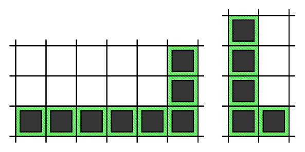
and three examples of invalid L-shapes.
Note that in the shape on the left, two segments do not share a common endpoint. The next two shapes do not meet the last requirement, as in the middle shape both segments have the same length, and in the last shape the longer segment is longer than twice the length of the shorter one.
Input
The first line of the input contains the number of test cases, $$$\mathbf{T}$$$. $$$\mathbf{T}$$$ test cases follow.
The first line of each testcase contains two integers $$$\mathbf{R}$$$ and $$$\mathbf{C}$$$.
Then, $$$\mathbf{R}$$$ lines follow, each line with $$$\mathbf{C}$$$ integers representing the cells of the grid.
Output
For each test case, output one line containing Case #$$$x$$$: $$$y$$$, where $$$x$$$ is
the test case number (starting from 1) and $$$y$$$ is the number of L-shapes.
Limits
Time limit: 60 seconds.
Memory limit: 1 GB.
$$$1 \le \mathbf{T} \le 100$$$.
Grid consists of $$$0$$$s and $$$1$$$s only.
Test Set 1
$$$1 \le \mathbf{R} \le 40$$$.
$$$1 \le \mathbf{C} \le 40$$$.
Test Set 2
$$$1 \le \mathbf{R} \le 1000$$$ and $$$1 \le \mathbf{C} \le 1000$$$ for at most $$$5$$$ test cases.
For the remaining cases, $$$1 \le \mathbf{R} \le 40$$$ and $$$1 \le \mathbf{C} \le 40$$$.
Sample
2
4 3
1 0 0
1 0 1
1 0 0
1 1 0
6 4
1 0 0 0
1 0 0 1
1 1 1 1
1 0 1 0
1 0 1 0
1 1 1 0
Case #1: 1
Case #2: 9
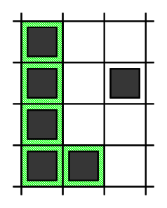
In Sample Case #1, there is one L-shape.
- The first one is formed by using cells: $$$(1,1)$$$, $$$(2,1)$$$, $$$(3,1)$$$, $$$(4,1)$$$, $$$(4,2)$$$
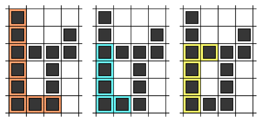
In Sample Case #2, there are nine L-shapes.
- The first one is formed by using cells: $$$(1,1)$$$, $$$(2,1)$$$, $$$(3,1)$$$, $$$(4,1)$$$, $$$(5,1)$$$, $$$(6,1)$$$, $$$(6,2)$$$, $$$(6,3)$$$
- The second one is formed by using cells: $$$(3,1)$$$, $$$(4,1)$$$, $$$(5,1)$$$, $$$(6,1)$$$, $$$(6,2)$$$
- The third one is formed by using cells: $$$(6,1)$$$, $$$(5,1)$$$, $$$(4,1)$$$, $$$(3,1)$$$, $$$(3,2)$$$
- The fourth one is formed by using cells: $$$(3,3)$$$, $$$(4,3)$$$, $$$(5,3)$$$, $$$(6,3)$$$, $$$(6,2)$$$
- The fifth one is formed by using cells: $$$(6,3)$$$, $$$(5,3)$$$, $$$(4,3)$$$, $$$(3,3)$$$, $$$(3,2)$$$
- The sixth one is formed by using cells: $$$(3,1)$$$, $$$(3,2)$$$, $$$(3,3)$$$, $$$(3,4)$$$, $$$(2,4)$$$
- The seventh one is formed by using cells: $$$(3,4)$$$, $$$(3,3)$$$, $$$(3,2)$$$, $$$(3,1)$$$, $$$(2,1)$$$
- The eighth one is formed by using cells: $$$(3,4)$$$, $$$(3,3)$$$, $$$(3,2)$$$, $$$(3,1)$$$, $$$(4,1)$$$
- The ninth one is formed by using cells: $$$(6,3)$$$, $$$(5,3)$$$, $$$(4,3)$$$, $$$(3,3)$$$, $$$(3,4)$$$
C. Rabbit House
Problem
Barbara got really good grades in school last year, so her parents decided to gift her with a pet rabbit. She was so excited that she built a house for the rabbit, which can be seen as a 2D grid with $$$\mathbf{R}$$$ rows and $$$\mathbf{C}$$$ columns.
Rabbits love to jump, so Barbara stacked several boxes on several cells of the grid. Each box is a cube with equal dimensions, which match exactly the dimensions of a cell of the grid.
However, Barbara soon realizes that it may be dangerous for the rabbit to make jumps of height greater than $$$1$$$ box, so she decides to avoid that by making some adjustments to the house. For every pair of adjacent cells, Barbara would like that their absolute difference in height be at most $$$1$$$ box. Two cells are considered adjacent if they share a common side.
As all the boxes are superglued, Barbara cannot remove any boxes that are there initially, however she can add boxes on top of them. She can add as many boxes as she wants, to as many cells as she wants (which may be zero). Help her determine what is the minimum total number of boxes to be added so that the rabbit's house is safe.
Input
The first line of the input gives the number of test cases, $$$\mathbf{T}$$$. $$$\mathbf{T}$$$ test cases follow.
Each test case begins with a line containing two integers $$$\mathbf{R}$$$ and $$$\mathbf{C}$$$.
Then, $$$\mathbf{R}$$$ lines follow, each with $$$\mathbf{C}$$$ integers. The $$$j$$$-th integer on $$$i$$$-th line, $$$\mathbf{G_{i,j}}$$$, represents how many boxes are there initially on the cell located at the $$$i$$$-th row and $$$j$$$-th column of the grid.
Output
For each test case, output one line containing Case #$$$x$$$: $$$y$$$,
where $$$x$$$ is the test case number (starting from 1) and $$$y$$$ is the minimum number
of boxes to be added so that the rabbit's house is safe.
Limits
Memory limit: 1 GB.
$$$1 \le \mathbf{T} \le 100$$$.
$$$0 \le \mathbf{G_{i,j}} \le 2 \cdot 10^6$$$, for all $$$i$$$, $$$j$$$.
Test Set 1
Time limit: 20 seconds.
$$$1 \le \mathbf{R}, \mathbf{C} \le 50$$$.
Test Set 2
Time limit: 40 seconds.
$$$1 \le \mathbf{R}, \mathbf{C} \le 300$$$.
Sample
3
1 3
3 4 3
1 3
3 0 0
3 3
0 0 0
0 2 0
0 0 0
Case #1: 0
Case #2: 3
Case #3: 4
In Sample Case #1, the absolute difference in height for every pair of adjacent cells is already at most $$$1$$$ box, so there is no need to add any extra boxes.
In Sample Case #2, the absolute difference in height of the left-most cell and the middle cell is $$$3$$$ boxes. To fix that, we can add $$$2$$$ boxes to the middle cell. But then, the absolute difference of the middle cell and the right-most cell will be $$$2$$$ boxes, so Barbara can fix that by adding $$$1$$$ box to the right-most cell. After adding these $$$3$$$ boxes, the safety condition is satisfied.
In Sample Case #3, the cell in the middle of the grid has an absolute difference in height of $$$2$$$ boxes with all of its four adjacent cells. One solution is to add exactly $$$1$$$ box to all of the middle's adjacent cells, so that the absolute difference between any pair of adjacent cells will be at most $$$1$$$ box. That requires $$$4$$$ boxes in total.
D. Checksum
Problem
Grace and Edsger are constructing a $$$\mathbf{N} \times \mathbf{N}$$$ boolean matrix $$$\mathbf{A}$$$. The element in $$$i$$$-th row and $$$j$$$-th column is represented by $$$\mathbf{A_{i,j}}$$$. They decide to note down the checksum (defined as bitwise XOR of given list of elements) along each row and column. Checksum of $$$i$$$-th row is represented as $$$\mathbf{R_i}$$$. Checksum of $$$j$$$-th column is represented as $$$\mathbf{C_j}$$$.
For example, if $$$\mathbf{N} = 2$$$, $$$\mathbf{A} = \begin{bmatrix} 1 & 0 \\ 1 & 1 \end{bmatrix}$$$, then $$$\mathbf{R} = \begin{bmatrix} 1 & 0 \end{bmatrix}$$$ and $$$\mathbf{C} = \begin{bmatrix} 0 & 1 \end{bmatrix}$$$.
Once they finished the matrix, Edsger stores the matrix in his computer. However, due to a virus, some of the elements in matrix $$$\mathbf{A}$$$ are replaced with $$$-1$$$ in Edsger's computer. Luckily, Edsger still remembers the checksum values. He would like to restore the matrix, and reaches out to Grace for help. After some investigation, it will take $$$\mathbf{B_{i,j}}$$$ hours for Grace to recover the original value of $$$\mathbf{A_{i,j}}$$$ from the disk. Given the final matrix $$$\mathbf{A}$$$, cost matrix $$$\mathbf{B}$$$, and checksums along each row ($$$\mathbf{R}$$$) and column ($$$\mathbf{C}$$$), can you help Grace decide on the minimum total number of hours needed in order to restore the original matrix $$$\mathbf{A}$$$?
Input
The first line of the input gives the number of test cases, $$$\mathbf{T}$$$. $$$\mathbf{T}$$$ test cases follow.
The first line of each test case contains a single integer $$$\mathbf{N}$$$.
The next $$$\mathbf{N}$$$ lines each contain $$$\mathbf{N}$$$ integers representing the matrix $$$\mathbf{A}$$$. $$$j$$$-th element on the $$$i$$$-th line represents $$$\mathbf{A_{i,j}}$$$.
The next $$$\mathbf{N}$$$ lines each contain $$$\mathbf{N}$$$ integers representing the matrix $$$\mathbf{B}$$$. $$$j$$$-th element on the $$$i$$$-th line represents $$$\mathbf{B_{i,j}}$$$.
The next line contains $$$\mathbf{N}$$$ integers representing the checksum of the rows. $$$i$$$-th element represents $$$\mathbf{R_i}$$$.
The next line contains $$$\mathbf{N}$$$ integers representing the checksum of the columns. $$$j$$$-th element represents $$$\mathbf{C_j}$$$.
Output
For each test case, output one line containing Case #$$$x$$$: $$$y$$$,
where $$$x$$$ is the test case number (starting from 1) and $$$y$$$ is the minimum number of hours to restore matrix $$$\mathbf{A}$$$.
Limits
Memory limit: 1 GB.
$$$1 \le \mathbf{T} \le 100$$$.
$$$-1 \le \mathbf{A_{i,j}} \le 1$$$, for all $$$i,j$$$.
$$$1 \le \mathbf{B_{i,j}} \le 1000$$$, for $$$i,j$$$ where $$$\mathbf{A_{i,j}} = -1$$$, otherwise $$$\mathbf{B_{i,j}} = 0$$$.
$$$0 \le \mathbf{R_i} \le 1$$$, for all $$$i$$$.
$$$0 \le \mathbf{C_j} \le 1$$$, for all $$$j$$$.
It is guaranteed that there exist at least one way to replace $$$-1$$$ in $$$\mathbf{A}$$$ with $$$0$$$ or $$$1$$$ such that $$$\mathbf{R}$$$ and $$$\mathbf{C}$$$ as satisfied.
Test Set 1
Time limit: 20 seconds.
$$$1 \le \mathbf{N} \le 4$$$.
Test Set 2
Time limit: 35 seconds.
$$$1 \le \mathbf{N} \le 40$$$.
Test Set 3
Time limit: 35 seconds.
$$$1 \le \mathbf{N} \le 500$$$.
Sample
3
3
1 -1 0
0 1 0
1 1 1
0 1 0
0 0 0
0 0 0
1 1 1
0 0 1
2
-1 -1
-1 -1
1 10
100 1000
1 0
0 1
3
-1 -1 -1
-1 -1 -1
0 0 0
1 1 3
5 1 4
0 0 0
0 0 0
0 0 0
Case #1: 0
Case #2: 1
Case #3: 2
In Sample Case #1, $$$\mathbf{A_{1,2}}$$$ can be restored using the checksum of either 1-st row or 2-nd column. Hence, Grace can restore the matrix without spending any time to recover the data.
In Sample Case #2, Grace spends one hour to recover $$$\mathbf{A_{1,1}}$$$. After that, she can use checksums of 1-st row and 1-st column to restore $$$\mathbf{A_{1,2}}$$$ and $$$\mathbf{A_{2,1}}$$$ respectively. And then she can use checksum of 2-nd row to restore $$$\mathbf{A_{2,2}}$$$. Hence, Grace can restore the matrix by spending one hour.
In Sample Case #3, Grace can spend one hour to recover $$$\mathbf{A_{1,1}}$$$ and another hour to recover $$$\mathbf{A_{2,2}}$$$. After that, she can use checksum to restore the rest of the matrix. Hence, Grace can restore the matrix by spending two hours in total.
Analysis — A. K-Goodness String
As per the given definition of operation, Ada can only change the goodness score by one in a single move. Therefore to get a string with the required goodness score in the minimum number of operations Ada can either increase or decrease the goodness score by one in each step. Let us assume there are $$$X$$$ indices($$$\le \mathbf{N}/2$$$ ($$$1$$$-indexed)) $$$i$$$ in the given string $$$\mathbf{S}$$$ such that $$$\mathbf{S}_i \neq \mathbf{S}_{\mathbf{N}-i+1}$$$. We have 3 cases now.
-
Case 1: $$$X = \mathbf{K}$$$,
In this case, Ada already has the string which has a goodness score of $$$\mathbf{K}$$$. Therefore number of operations required is $$$0$$$. -
Case 2: $$$X > \mathbf{K}$$$,
In this case, Ada can change $$$(X-\mathbf{K})$$$ letters at indices $$$i$$$ ($$$1 ≤ i ≤ \mathbf{N}/2$$$ ($$$1$$$-indexed)) that satisfy $$$\mathbf{S}_i \neq \mathbf{S}_{\mathbf{N}-i+1}$$$ to the letter at $$$\mathbf{S}_{\mathbf{N}-i+1}$$$. Then she will have a string with a goodness score of $$$\mathbf{K}$$$. Therefore the minimum number of operations is $$$(X-\mathbf{K})$$$. -
Case 3: $$$X < \mathbf{K}$$$,
In this case, Ada can change $$$(\mathbf{K}-X)$$$ letters at indices $$$i$$$ ($$$1 ≤ i ≤ \mathbf{N}/2$$$ ($$$1$$$-indexed)) that satisfy $$$\mathbf{S}_i = \mathbf{S}_{\mathbf{N}-i+1}$$$ to any other uppercase letter other than the one at $$$\mathbf{S}_{\mathbf{N}-i+1}$$$. As a result, she will have a string with a goodness score of $$$\mathbf{K}$$$. Therefore the minimum number of operations is $$$(\mathbf{K}-X)$$$.
All the above described operations can be done in $$$O(\mathbf{N})$$$ complexity. Therefore the overall complexity is $$$O(\mathbf{N})$$$.
Sample Code (C++)
int kGoodnessString(string s, int k) {
  int minOperations = 0, x = 0;
  for(int i = 0; i < s.size() / 2; i++) {
     if(s[i] != s[s.size() - i - 1]) {
         x++;
     }
  }

  if(x == k) {
      minOperations = 0;
  }
  else if(x > k) {
      minOperations = x - k;
  }
  else {
      minOperations = k - x;
  }
  return minOperations;
}
Analysis — B. L Shaped Plots
Test set 1
In order to verify that a segment is good, we need to check whether all the cells in that segment contain $$$1$$$ or not. To check whether all the cells in a segment contain $$$1$$$ or not, we can calculate prefix sum of the matrix and then check whether sum of cells on this segment is equal to the length of the segment or not. Let $$$query(a,b,c,d)$$$ denote the sum of cells in submatrix with $$$(a,b)$$$ as top left corner and $$$(c,d)$$$ as bottom right corner. We can calculate this sum in $$$O(1)$$$ using the prefix sum matrix. For more details on using prefix sum to calculate sum of cells on a submatrix, please refer this. In order to get the sum of cells on segment from $$$(i,j)$$$ to $$$(i,l)$$$, we can simply check if $$$query(i,j,i,l) = |j-l|+1$$$.
L-shape comprises of two segments which meet at a common point. Except the common point, consider the other end point of one segment as $$$(i,j)$$$ and the end point of the other segment as $$$(k,l)$$$. Now these end points could meet at either $$$(i,l)$$$ or $$$(k,j)$$$ to form an L-shape. So, if we know the end points of each segment, we can figure out the common point where segments would meet.
For each pair of end points $$$(i,j)$$$ and $$$(k,l)$$$ of segments of L-shape, we already saw that there could be $$$2$$$ possible meeting points.
- For segments meeting at $$$(i,l)$$$, check that $$$query(i,j,i,l) = |j-l|+1$$$ and $$$query(k,l,i,l) = |i-k|+1$$$. Besides, either $$$|j-l|+1 = 2 \times (|i-k|+1)$$$ or $$$|i-k|+1= 2 \times (|j-l|+1)$$$ should be true. If these conditions are satisfied, increase the answer by $$$1$$$.
- For segments meeting at $$$(k,j)$$$, check that $$$query(i,j,k,j) = |i-k|+1$$$ and $$$query(k,l,k,j) = |j-l|+1$$$. Besides, either $$$|i-k|+1 = 2 \times (|j-l|+1)$$$ or $$$|j-l|+1= 2 \times (|i-k|+1)$$$ should be true. If these conditions are satisfied, increase the answer by $$$1$$$.
We can iterate over all possible end points of these two segments L-shape because there are $$$O(\mathbf{R}^{2} \times \mathbf{C}^{2})$$$ such possible combinations. We can calculate the number of possible L-shapes with these end points in $$$O(1)$$$. Hence, the overall complexity of the solution is $$$O(\mathbf{R}^{2} \times \mathbf{C}^{2})$$$.
Test set 2
We cannot iterate over all possible end points of the segments for this test set as the solution would time out. If for each cell, we can quickly calculate how many L-shapes are such that both of its segments meet at this cell, we can iterate over each cell of the matrix only once and calculate our answer. We can safely ignore those cells that have value 0 as they cannot be part of any L-shape.
Consider a cell $$$(i,j)$$$. There can be 4 types of L-shapes that have both of its segments meet this cell.
- Type 1: One of the segments is to top of $$$(i,j)$$$, and other segment is to the right of $$$(i,j)$$$.
- Type 2: One of the segments is to top of $$$(i,j)$$$, and other segment is to the left of $$$(i,j)$$$.
- Type 3: One of the segments is to bottom of $$$(i,j)$$$, and other segment is to the right of $$$(i,j)$$$.
- Type 4: One of the segments is to bottom of $$$(i,j)$$$, and other segment is to the left of $$$(i,j)$$$.
Let $$$Count(x,y)$$$ be the number of L-shapes with both its segments meeting at a particular point of which the length of the segment parallel to one axis is $$$x$$$ and the length of the segment parallel to the other axis is $$$y$$$. Number of L-shapes with longer segment as part of the segment with length $$$x$$$ are $$$min(\frac{x}{2},y) - 1$$$. Similarly, number of L-shapes with longer segment as part of the segment with length $$$y$$$ are $$$min(\frac{y}{2},x) - 1$$$. Hence, $$$Count(x,y) = min(\frac{x}{2},y) + min(\frac{y}{2},x) - 2$$$.
If we can calculate number of consecutive cells that have value 1 in each side of $$$(i,j)$$$, we can calculate number of L-shapes of each type with this cell as the common endpoint of the segments using the $$$Count()$$$ function above. Let $$$top(i,j)$$$ denote the number of consecutive cells that have value 1 including $$$(i,j)$$$ and cells above it. For cells with value 0, $$$top(i,j) = 0$$$. Formally for cells with value 1, $$$top(i,j) = i - k + 1$$$ where $$$1 \le k \le i$$$ and k is least possible value such that all cells from $$$(k,j)$$$ to $$$(i,j)$$$ have value 1. Similarly, we can define $$$bottom(i,j)$$$, $$$left(i,j)$$$ and $$$right(i,j)$$$ denoting maximum number of consecutive cells on bottom, left and right of $$$(i,j)$$$ respectively.
We can calculate $$$top(i,j)$$$ and $$$left(i,j)$$$ by iterating from the starting of the matrix and updating their values. Refer to the code below to calculate these values.
  for(int i = 1; i <= R; i++) {
    for(int j = 1; j <= C; j++) {
       if (matrix[i][j] == 0) continue;
       top[i][j] = top[i - 1][j] + 1;
       left[i][j] = left[i][j - 1] + 1;
    }
 }
Similarly, we can calculate $$$bottom(i,j)$$$ and $$$right(i,j)$$$ by iterating from the end of the matrix. After knowing these values, we can calculate number of L-shapes of each type for cell $$$(i,j)$$$. $$$Count(top(i,j), right(i,j))$$$, $$$Count(top(i,j), left(i,j))$$$, $$$Count(bottom(i,j), right(i,j))$$$ and $$$Count(bottom(i,j), left(i,j))$$$ denote the number of L-shapes of type 1, 2, 3 and 4 respectively. Thus, for each cell we can add $$$Count(top(i,j), left(i,j)) + Count(top(i,j), right(i,j)) + Count(bottom(i,j), left(i,j)) + Count(bottom(i,j), right(i,j))$$$ to the answer.
$$$top(i,j)$$$, $$$bottom(i,j)$$$, $$$left(i,j)$$$ and $$$right(i,j)$$$ can be calculated in $$$O(\mathbf{R} \times \mathbf{C})$$$ time complexity. $$$Count(i,j)$$$ can be calculate in $$$O(\mathbf{R} \times \mathbf{C})$$$ time complexity. Finally, we need to iterate over each cell of the matrix, and we can update the answer in $$$O(1)$$$ for each cell. Thus, the overall complexity of the solution is $$$O(\mathbf{R} \times \mathbf{C})$$$.
Analysis — C. Rabbit House
Barbara is given a 2D grid with $$$\mathbf{R}$$$ rows and $$$\mathbf{C}$$$ columns. Her goal is to create a grid such that no two adjacent cells have an absolute difference in height greater than $$$1$$$. Moreover, she is only allowed to increase the height of cells.
We notice that the cell initially with the largest height ($$$H$$$) never requires increasing. Furthermore, Barbara can update its neighbor cells to have a height of $$$H - 1$$$ (unless they already have a height of $$$H$$$). Afterwards, she can repeat the process for the cell with the next largest height, until she visits all the cells.
One thing to be careful of in this problem is that the final result can be larger than the limits of a 32-bit integer. Using 64-bit integers avoids WAs due to overflow.
Test set 1
For this test set, Barbara sees that $$$1 \le \mathbf{R}, \mathbf{C} \le 50$$$. Therefore, she performs a linear scan over the grid to find the cell with the largest height. Then, she updates the height of its neighbors, and increments the result to account for the increase in height.
Finally, she marks this cell as visited, which can be done via a secondary 2D grid of booleans. She repeats the above process until all cells have been visited, and return the result.
The linear scan can be done in $$$O(\mathbf{R} \cdot \mathbf{C})$$$, and Barbara visits each cell exactly once, so she
performs the linear scan $$$O(\mathbf{R} \cdot \mathbf{C})$$$ times. The overall time complexity is therefore
$$$O((\mathbf{R} \cdot \mathbf{C})^2)$$$. This fits within the limits of the small test set.
The additional space complexity is $$$O(\mathbf{R} \cdot \mathbf{C})$$$ due to the secondary 2D grid of
booleans.
Test set 2
For this test set, $$$1 \le \mathbf{R}, \mathbf{C} \le 300$$$. A time complexity of $$$O((\mathbf{R} \cdot \mathbf{C})^2)$$$ will not satisfy the time limits.
Barbara still needs to visit the unvisited cell with the largest height in each iteration. However, this can be done in $$$O(\log(\mathbf{R} \cdot \mathbf{C}))$$$ using a priority queue. In each iteration, she pops the cell with the largest height, updates the height of its neighbors in the priority queue, and increments the result.
The time complexity of the above solution is $$$O(\mathbf{R} \cdot \mathbf{C} \cdot \log(\mathbf{R} \cdot \mathbf{C}))$$$. The additional space complexity is still $$$O(\mathbf{R} \cdot \mathbf{C})$$$, since initially the priority queue contains all the cells.
Note that, depending on the implementation, updating a non-top element in the priority queue might not be an $$$O(1)$$$ operation. In such cases, one trick would be to insert a new element into the queue with the new height, and update the height in the grid. On processing any element, check whether the height in the queue corresponds to the height in the grid, and ignore the element otherwise. This does not change the worst-case time and space complexity, since the maximum number of times a cell can be added to the queue is $$$4$$$.
Further Improvements
While not necessary to pass the time limits, the time complexity can be reduced further.
One approach is to replace the priority queue with a list of buckets, each bucket containing a set of cells with a given height. With this approach, Barbara can iterate over the buckets in decreasing order of height in order to visit each cell, then apply the same algorithm as above: update the neighbors (by placing them in their new buckets according to their new height), and remove the visited cells from the list.
By using a hashset for each bucket, insertion and removal becomes an $$$O(1)$$$ operation. She can also use a vector. However, the trick from Test Set 2 is needed to maintain an $$$O(1)$$$ insertion/removal in that case. Iterating over the buckets is linear in the number of buckets, and she will visit at most $$$O(\mathbf{R} \cdot \mathbf{C})$$$ cells.
Let $$$G = \max(\mathbf{G_{i,j}})$$$. Since no cell has an initial height larger than $$$G$$$, and she will never increase the height of the cell with the largest height, she observes that the number of buckets is at most $$$G$$$. This leads to a time complexity of $$$O(\mathbf{R} \cdot \mathbf{C} + G)$$$.
Barbara can improve this further. Notice that all cells in the final grid will have a height of at least $$$G - \mathbf{R} - \mathbf{C} + 2$$$. She achieves this value by decreasing the height by 1 with each step away from the highest cell. The maximum number of steps occurs when the highest cell is in a corner of the grid: the opposite corner is $$$\mathbf{R} + \mathbf{C} - 2$$$ steps away.
Now, she can first increase the height of all cells to $$$G - \mathbf{R} - \mathbf{C} + 2$$$, then apply the same bucketing approach. Except, now the number of buckets is $$$\mathbf{R} + \mathbf{C} - 2$$$, leading to a time complexity of $$$O(\mathbf{R} \cdot \mathbf{C} + \mathbf{R} + \mathbf{C}) = O(\mathbf{R} \cdot \mathbf{C})$$$.
Analysis — D. Checksum
Suppose we know a subset $$$S$$$ of elements of the matrix $$$\mathbf{A}$$$ because they are either given in the input or revealed by Edsger. Can we restore the remaining elements? If there is only one unknown element in some row or column, we can recover its true value from the known elements in that row or column and the respective checksum. We can apply such an element recovery step until all elements are known or we end up with a matrix where each row and column has at least two unknown elements (aside from fully reconstructed rows and columns). It will be shown later that the whole matrix can be restored using this simple strategy or the subset $$$S$$$ does not provide enough information to do so.
Test Set 1
For the small test set, we can examine every potential subset $$$S$$$ of matrix elements and check if $$$S$$$ is sufficient to restore the whole matrix. Among all sufficient subsets $$$S$$$, we pick the smallest in terms of hours as our answer.
Given a subset $$$S$$$ of known elements, the above matrix recovery strategy can be implemented in $$$O(\mathbf{N}^2)$$$ time. For example, we can use a BFS-like algorithm iterating over a queue of elements that are the only unknown elements in their rows or columns and calculating their true values one by one. For the sake of efficiency, we also need to maintain the XOR values of currently known elements for each row and column as well as the number of unknown elements per each row and column. As soon as the number of unknown elements for a row or column becomes $$$1$$$, we add that element to the queue.
There are $$$O(2^{\mathbf{N}^2})$$$ subsets of elements. Consequently, the overall time complexity of this brute-force algorithm is $$$O(2^{\mathbf{N}^2} \times \mathbf{N}^2)$$$.
Test Set 2
Let us look at our problem from graphs perspective. Namely, we construct a weighted bipartite graph $$$G$$$, where the rows and columns of the matrix $$$\mathbf{A}$$$ are represented by nodes in $$$G$$$, and there is an edge of weight $$$\mathbf{B_{i,j}}$$$ between $$$i$$$-th row and $$$j$$$-th column if and only if $$$\mathbf{A_{i,j}} = -1$$$. Please see the below example to make the construction more clear.
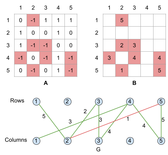
An isolated node represents a row or column with all its elements known. We can safely disregard such nodes. A leaf node with exactly one incident edge represents a row or column with precisely one unknown element. Note that the process outlined in the first paragraph corresponds to repeated removal of leaves from the graph. If we end up with an empty graph in this way, it means that the original graph must have been a forest without any cycles and we can recover the full matrix without spending any time.
So what if the graph $$$G$$$ does contain a cycle? Given any assignment of binary values to the elements of the matrix, we can flip the values of elements corresponding to the edges of a cycle, and this operation would not change the XOR checksum of any row or column. Consequently, we cannot tell the true value of elements on a cycle unless we reveal at least one of them, and effectivelly break the cycle by removing the edge from the graph and paying a delicious price. In other words, in order to be able to recover the whole matrix, it is necessary to break all cycles by revealing and removing some edges. It is also sufficient — once all cycles have been broken, what remains is a forest of edges, and the true value of all remaining edges can be determined unambiguously.
Thus we have reduced the original problem to finding a minimum weight subset of edges that breaks all cycles. An intuitive greedy approach involves iterating over the edges in a non-decreasing order of weights and removing the current edge from the graph if it is part of a cycle. An edge is part of a cycle if there is a simple path between its end-nodes other than the edge itself — a condition that can be tested by, say, running a depth-first search from one of the end-nodes.
In our example above, once we remove the cheapest edge of cost $$$1$$$ (the red edge), what remains is a tree, so no other edges will be removed.
Since there can be up to $$$\mathbf{N}^2$$$ edges, the above steps are repeated $$$O(\mathbf{N}^2)$$$ times. One run of the depth-first search costs $$$O(\mathbf{N}^2)$$$ time as well, so the overall time complexity of this approach is $$$O(\mathbf{N}^4)$$$.
But what about the correctness of this greedy approach? The proof is very similar to that of Kruskal's algorithm. Consider the first edge $$$e$$$ that is removed by the algorithm, so it has the smallest weight among all edges on cycles. In particular, suppose that $$$e$$$ is part of a cycle $$$C$$$. Now, consider any cycle breaking set of edges $$$X$$$ that does not include $$$e$$$. Since the cycle $$$C$$$ must be broken, $$$X$$$ must contain an edge $$$f \neq e$$$ that is also part of the cycle $$$C$$$. The set of edges $$$Y = X - f + e$$$ has a total weight no larger than the weight of $$$X$$$ and it is cycle breaking as well. To prove the second claim, assume the contrary that the graph $$$G - Y$$$ contains a cycle $$$C'$$$, which necessarily includes the edge $$$f$$$ and does not include the edge $$$e$$$. But then we can combine the paths $$$P = C - f$$$ and $$$P' = C' - f$$$ to form a cycle in $$$G - X$$$, which contradicts the fact that $$$X$$$ was cycle breaking. It follows that the edge $$$e$$$ is part of some optimal solution and our greedy choice was valid.
Test Set 3
Of course, the problem of finding a minimum weight cycle breaking edge set is equivalent to the well known problem of finding a maximum weight spanning forest of $$$G$$$, except that we would build the complement set of edges to keep rather than the set of edges to remove. In the example above, the edges of the maximum weight spanning forest are rendered green. It would cost Grace one hour (the red edge) to reconstruct the whole matrix.
The graph may potentially have up to $$$\mathbf{N}^2$$$ edges, therefore, a simple implementation of Prim's algorithm without maintaining a priority queue data structure would achieve an $$$O(\mathbf{N}^2)$$$ time complexity. Note that because of the high density of the graph, Prim's algorithm is a better choice than Kruskal's algorithm, as the later would need $$$O(\mathbf{N}^2 \times \log \mathbf{N})$$$ time for sorting the edges.
It is interesting to note that we never use the actual checksums in the graph construction nor the maximum spanning forest algorithm, therefore, the input values $$$\mathbf{R_i}$$$ and $$$\mathbf{C_i}$$$ can be safely ignored.