Google Code Jam Archive — Code Jam to I/O for Women 2022 problems
Overview
Code Jam to I/O for Women returned for its ninth year. The round started with Inversions Organize, helping the I/O marketing team balance an advertising display. Ingredient Optimization followed where a greedy strategy could help Hathai use her Thai Basil leaves optimally to serve the most customers. Next, things ramped up with Interesting Outing which was a hit for anyone who likes to travel. Learning about diameters of a tree would help one solve this problem. Finally, Inventor Outlasting closed out the set with a game between two friends personifying theme park attraction inventors. You might see theme parks reappear in the future!
SoulTch was the first one to achieve a perfect score and landed at the top of the scoreboard once the round concluded. limli came in second place solving the set only 34 seconds later, and damndelion rounded out the top 3. In total, 4 people managed a perfect score. More than 1800 people scored points out of 3243 participants that submitted a solution.
We hope you enjoyed Code Jam to I/O for Women 2022 and learned a new thing or two while participating. Congratulations to those in the top 150! You will receive Google I/O branded swag, access to invite-only virtual events, as well as a $150 USD stipend to enhance your I/O viewing experience. The Code Jam to I/O for Women team will contact you soon with more information about your prize.
We look forward to seeing you on the scoreboard in 2023. Until then, Code Jam's Qualification Round will kick off on April 1. Hone your coding skills and get ready for the competition next year with Kick Start, which offers challenges throughout the year.
Cast
Inversions Organize: Written by Melisa Halsband. Prepared by Salma Mustafa.
Ingredient Optimization: Written by Sumedha Agarwal. Prepared by Michelle Wang.
Interesting Outing: Written by Frances Cooper. Prepared by Chu-ling Ko.
Inventor Outlasting: Written by Claire Yang. Prepared by Chun-nien Chan.
Solutions and other problem preparation and review by Balganym Tulebayeva, Bianca Oe, Chakradhar Reddy, Chu-ling Ko, Chun-nien Chan, Daria Tupikina, Deeksha Kaurav, Harshada Kumbhare, Hsin-Yi Wang, Jitesh Yadav, Lizzie Sapiro Santor, Maneeshita Sharma, Marina Vasilenko, Mary Yang, Melisa Halsband, Michelle Wang, Pablo Heiber, Sadia Atique, Samiksha Gupta, Sarah Young, Sasha Fedorova, Sona Mehra, Sreya Mittal, Sumedha Agarwal, Timothy Buzzelli, Vivian Tsai, and Wendi Wang.
Analysis authors:
- Inversions Organize: Sarah Young.
- Ingredient Optimization: Salma Mustafa.
- Interesting Outing: Sadia Atique.
- Inventor Outlasting: Chu-ling Ko.
A. Inversions Organize
Problem
After the troubles with printing advertising for IO two years ago, the marketing team of the
conference decided to use an interactive installation. It consists of a matrix of $$$2\mathbf{N}$$$
rows and $$$2\mathbf{N}$$$ columns of touchscreens. Each touchscreen can display either an uppercase
I or an uppercase O. When one of the screens is touched, it switches
the letter it displays to the one it was not displaying right before the touch occurred.
You are looking at one of those installations, and find it to be disorganized. You want to
change some of the letters such that the top $$$\mathbf{N}$$$ rows show the same number of letter
I's as the bottom $$$\mathbf{N}$$$ rows, and at the same time, the leftmost $$$\mathbf{N}$$$ columns
show the same number of letter I's in total as the rightmost $$$\mathbf{N}$$$ columns.
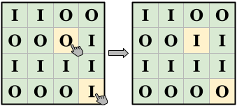
For example, in the left picture above, $$$\mathbf{N}=2$$$. The top $$$2$$$ rows show $$$3$$$ letter
I's in total, while the bottom $$$2$$$ rows show $$$5$$$. On the other hand,
both the leftmost $$$2$$$ columns and the rightmost $$$2$$$ columns show $$$4$$$ letter
I's. By touching the two highlighted screens we can change the state to that
shown in the right picture, which shows $$$4$$$ letter I's in the top $$$2$$$
columns and in the bottom $$$2$$$ columns, and also maintains the balance between the left
and right sides.
Given the state of the installation, can you find the minimum number of letter changes needed to achieve your organizational goal?
Input
The first line of the input gives the number of test cases, $$$\mathbf{T}$$$. $$$\mathbf{T}$$$ test cases follow. Each test case starts with a line containing a single integer $$$\mathbf{N}$$$, half the number of rows and columns of the matrix. Then, $$$2\mathbf{N}$$$ lines follow. The $$$i$$$-th of these contains a string of $$$2\mathbf{N}$$$ characters $$$\mathbf{C_{i,1}}\mathbf{C_{i,2}}\cdots\mathbf{C_{i,2N}}$$$. $$$\mathbf{C_{i,j}}$$$ is the letter currently displayed in the screen in the $$$i$$$-th row and $$$j$$$-th column of the matrix.
Output
For each test case, output one line containing Case #$$$x$$$: $$$y$$$,
where $$$x$$$ is the test case number (starting from 1) and $$$y$$$ is the minimum number of
touches required to make the installation simultaneously display the same number of letter
I's in its top and bottom halves, and the same number of letter
I's in its left and right halves.
Limits
Time limit: 20 seconds.
Memory limit: 1 GB.
$$$1 \le \mathbf{T} \le 100$$$.
$$$\mathbf{C_{i,j}}$$$ is either an uppercase I or an uppercase O,
for all $$$i, j$$$.
Test Set 1 (Visible Verdict)
$$$1 \le \mathbf{N} \le 2$$$.
Test Set 2 (Hidden Verdict)
$$$1 \le \mathbf{N} \le 100$$$.
Sample
3
2
IIOO
OOOI
IIII
OOOI
1
IO
OO
2
OIOI
IOIO
OIOI
IOIO
Case #1: 2
Case #2: 1
Case #3: 0
Sample Case #1 is the one explained in the statement. Not touching anything does not work,
and a single touch would leave an odd number of letters I in total, so the
result cannot be balanced. It is explained in the statement how it can be balanced with
two touches (there are other ways).
In Sample Case #2, changing the top left corner to O leaves no letter I,
so all halves have the same amount ($$$0$$$).
In Sample Case #3, the installation is already organized according to your requirements, so no touch is needed.
B. Ingredient Optimization
Problem
Hathai is proud that her catering service provides the freshest food in town. To accomplish that, she gets fresh ingredients with no preservatives delivered constantly. This brings about the challenge of preventing the ingredients from spoiling. Her current special uses exactly $$$\mathbf{U}$$$ leaves of Thai basil, that need special care.
Hathai has the schedule of the deliveries of Thai basil. The $$$i$$$-th delivery comes at the beginning of time $$$\mathbf{M_i}$$$ (in minutes since opening time), and brings exactly $$$\mathbf{L_i}$$$ leaves of Thai basil that can be stored for at most $$$\mathbf{E_i}$$$ minutes since arriving. Hathai has orders to prepare her specialty dish at times $$$\mathbf{O_1}, \mathbf{O_2}, \dots, \mathbf{O_N}$$$. Order $$$i$$$ can only be fulfilled if she has $$$\mathbf{U}$$$ unspoiled leaves of Thai basil at time $$$\mathbf{O_i}$$$. Note that if leaves would spoil at the same time an order comes in, those leaves cannot be used to fulfill that order. If an order is fulfilled, $$$\mathbf{U}$$$ of the leaves available have to be used and cannot be used for future orders. Once Hathai gets an order that she cannot fulfill, all of the remaining orders will also be canceled because she needs to close her kitchen and think about how to improve the fulfillment schedule.
For example, suppose Hathai's schedule has the following $$$4$$$ deliveries:
- Delivery time: $$$1$$$. Amount: $$$10$$$. Time remaining until spoiled: $$$2$$$.
- Delivery time: $$$3$$$. Amount: $$$4$$$. Time remaining until spoiled: $$$2$$$.
- Delivery time: $$$5$$$. Amount: $$$1$$$. Time remaining until spoiled: $$$4$$$.
- Delivery time: $$$10$$$. Amount: $$$6$$$. Time remaining until spoiled: $$$3$$$.
The first delivery become spoiled at time $$$3$$$, so it cannot be used on any order. Then the first order and the second order at time $$$3$$$ and time $$$4$$$ can be fulfilled and use up the $$$4$$$ leaves from the second delivery. For the third order at time $$$6$$$, there is only $$$1$$$ leaf in the storage, so Hathai cannot fulfill this order. Note that although there is a delivery at time $$$10$$$, she still cannot fulfill the fourth order at time $$$10$$$ because she has already closed her kitchen. In this example, Hathai managed to fulfill $$$2$$$ orders in total.
Given the delivery and order schedules, find out the maximum number of orders Hathai can fulfill if she optimizes the use of the Thai basil leaves.
Input
The first line of the input gives the number of test cases, $$$\mathbf{T}$$$. $$$\mathbf{T}$$$ test cases follow. Each test case starts with a line containing three integers $$$\mathbf{D}$$$, $$$\mathbf{N}$$$, and $$$\mathbf{U}$$$: the number of deliveries, the number of orders and the amount of leaves needed for each order, respectively. Then, $$$\mathbf{D}$$$ lines follow. The $$$i$$$-th of these lines contains three integers $$$\mathbf{M_i}$$$, $$$\mathbf{L_i}$$$, and $$$\mathbf{E_i}$$$: the time of the delivery in minutes since opening time, the amount of Thai basil leaves delivered, and the number of minutes those leaves can be stored and remain fresh, respectively, of the $$$i$$$-th delivery. Then, the last line contains $$$\mathbf{N}$$$ integers $$$\mathbf{O_1}, \mathbf{O_2}, \dots, \mathbf{O_N}$$$, where $$$\mathbf{O_j}$$$ is the time, in minutes since opening time, at which the $$$j$$$-th order must be prepared.
Output
For each test case, output one line containing Case #$$$x$$$: $$$y$$$,
where $$$x$$$ is the test case number (starting from 1) and $$$y$$$ is an integer
representing the maximum number of orders Hathai can fulfill.
Limits
Time limit: 5 seconds.
Memory limit: 1 GB.
$$$1 \le \mathbf{T} \le 100$$$.
$$$1 \le \mathbf{D} \le 100$$$.
$$$1 \le \mathbf{N} \le 100$$$.
$$$1 \le \mathbf{U} \le 100$$$.
$$$1 \le \mathbf{M_i} \le 10^9$$$, for all $$$i$$$.
$$$\mathbf{M_i} \lt \mathbf{M_{i+1}}$$$, for all $$$i$$$. (Deliveries are given in increasing order of time.)
$$$1 \le \mathbf{L_i} \le 100$$$, for all $$$i$$$.
$$$1 \le \mathbf{O_j} \le 10^9$$$, for all $$$j$$$.
$$$\mathbf{O_j} \lt \mathbf{O_{j+1}}$$$, for all $$$j$$$. (Orders are given in increasing order of time.)
Test Set 1 (Visible Verdict)
$$$\mathbf{E_i} = 10^9$$$, for all $$$i$$$. (No Thai basil leaf expires before an order comes.)
Test Set 2 (Hidden Verdict)
$$$1 \le \mathbf{E_i} \le 10^9$$$, for all $$$i$$$.
Sample
Note: there are additional samples that are not run on submissions down below.2 2 4 5 20 8 1000000000 60 4 1000000000 10 30 50 70 3 5 5 20 8 1000000000 50 3 1000000000 60 100 1000000000 30 50 59 70 90
Case #1: 0
Case #2: 2
In Sample Case #1, Hathai cannot fulfill the first order, because it came too early, before any deliveries brought in Thai leaves. So she has to close her kitchen immediately without fulfilling any order.
In Sample Case #2, Hathai can fulfill the first order, and her second delivery arrives just in time to help her fulfill the second order. However, the huge third delivery does not get to her in time to help her with the third order, so that one goes unfulfilled and so do the remaining ones.
Additional Sample - Test Set 2
The following additional sample fits the limits of Test Set 2. It will not be run against your submitted solutions.1 4 4 2 1 10 2 3 4 2 5 1 4 10 6 3 3 4 6 10
Case #1: 2
This additional sample is the one explained in the problem statement.
C. Interesting Outing
Problem
You are hosting visitors from out of town, and want to take them out and show them the most interesting places in town.
There are $$$\mathbf{N}$$$ interesting sights you want to tour. You have identified $$$\mathbf{N}-1$$$ interesting methods of transportation. Each method of transportation bidirectionally connects a pair of sights. Luckily, there is exactly one way to get from any interesting sight to another without using any transportation method more than once.
You know how much it would cost for the group to use each transportation method one time (you pay once per use). You can decide the starting and ending sights of the tour (they can be the same or different sights). You do not need to worry about the cost of getting to the starting point nor coming back from the ending point, only the cost of transportation between sights during the tour. What is the cheapest way to see all sights at least once each?
Input
The first line of the input gives the number of test cases, $$$\mathbf{T}$$$. $$$\mathbf{T}$$$ test cases follow. Each test case starts with a line containing a single integer $$$\mathbf{N}$$$, the number of sights you want to tour. Then, $$$\mathbf{N}-1$$$ lines follow. The $$$i$$$-th of these lines contains three integers $$$\mathbf{A_i}$$$, $$$\mathbf{B_i}$$$, and $$$\mathbf{C_i}$$$, representing that the $$$i$$$-th method of transportation can take your group from sight $$$\mathbf{A_i}$$$ to sight $$$\mathbf{B_i}$$$ or from sight $$$\mathbf{B_i}$$$ to sight $$$\mathbf{A_i}$$$ for a cost of $$$\mathbf{C_i}$$$ coins per usage.
Output
For each test case, output one line containing Case #$$$x$$$: $$$y$$$,
where $$$x$$$ is the test case number (starting from 1) and $$$y$$$ is an integer
representing the minimum cost of a tour that visits each sight at least once.
Limits
Time limit: 10 seconds.
Memory limit: 1 GB.
$$$1 \le \mathbf{T} \le 100$$$.
$$$1 \le \mathbf{A_i} \lt \mathbf{B_i} \le \mathbf{N}$$$, for all $$$i$$$.
It is possible to travel between any pair of sights using only the methods of transportation
given in the input. (This and the previous limits imply the sights and transportation
methods form an unrooted
tree.)
$$$1 \le \mathbf{C_i} \le 10^9$$$ for all $$$i$$$.
Test Set 1 (Visible Verdict)
$$$2 \le \mathbf{N} \le 10$$$.
Test Set 2 (Hidden Verdict)
$$$2 \le \mathbf{N} \le 1000$$$.
Sample
3
6
1 3 10
4 5 10
3 4 10
4 6 20
2 3 30
6
1 3 35
4 5 10
3 4 10
4 6 20
2 3 30
5
1 3 1000000000
2 3 1000000000
3 4 1000000000
3 5 1000000000
Case #1: 100
Case #2: 145
Case #3: 6000000000
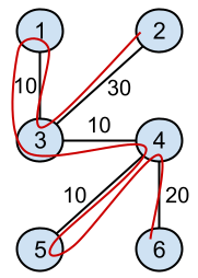
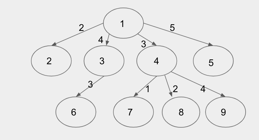
In Sample Case #1 (as seen below), an optimal route (marked with a red line in the picture above) goes through the following sights: $$$2, 3, 1, 3, 4, 5, 4, 6$$$.
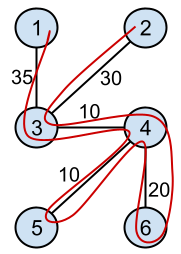
In Sample Case #2 (as seen above), the only change compared with the setup in Sample Case #1 is that the transportation between sights $$$1$$$ and $$$3$$$ got more expensive: from $$$10$$$ to $$$35$$$. The route $$$2, 3, 1, 3, 4, 5, 4, 6$$$ costs $$$150$$$ in this scenario and it is not optimal. The optimal route is $$$2, 3, 4, 6, 4, 5, 4, 3, 1$$$ instead (also marked in red in the picture).
Notice in Sample Case #3 that the answer may be larger than $$$2^{32}$$$.
D. Inventor Outlasting
Problem
Izabella and Olga are playing a new game alternating turns. In this game, they personify attraction inventors working for a theme park. The board is a matrix of square cells that illustrates the map of the theme park. Some cells were deemed apt to host a new attraction.
When an attraction is built, signs to advertise it are added automatically. $$$4$$$ sign builders are sent in each diagonal direction. The one moving towards the north-east direction proceeds as follows: starting at the cell where the location is built, check the cell north-east from its current cell. If there is no cell there, or the cell is occupied, they stop. Otherwise, they move to that cell, build a sign there, and repeat. Sign builders that move in the north-western, south-eastern and south-western directions proceed the same, except for the direction of the movements. A cell is considered occupied if it contains either an attraction or a sign.
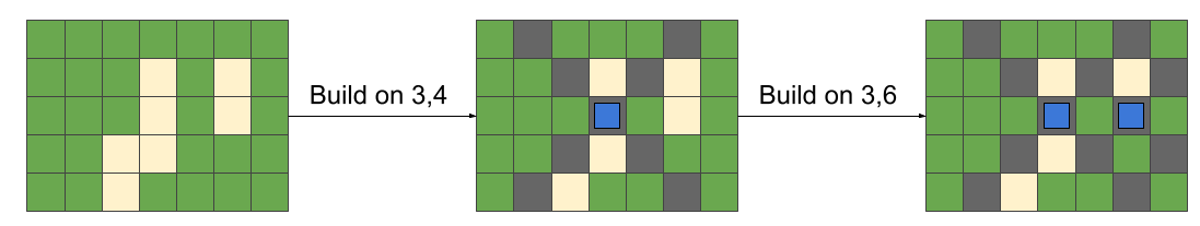
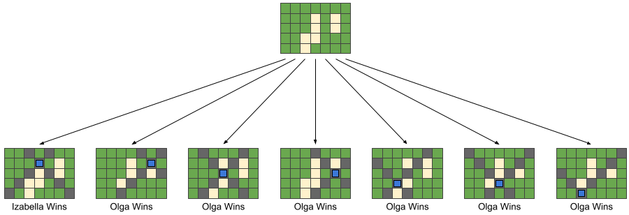
For example, suppose the left picture below represents a map, with yellow cells representing the
spots where attractions can be built. After an attraction is built on $$$3,4$$$ of the map
(now marked with a blue square), signs are also built on cells marked in gray.
Some spots that were previously available for attractions are no longer available because they
contain a sign now. Notice after a second attraction is built on $$$3,6$$$, the new sign builders
only move as far as a previous sign, leading to the situation illustrated in the right picture.
In a turn, a player can choose to build an attraction in any available spot, and then the sign builders proceed automatically, possibly invalidating other spots as in the example. The goal of the game is to outlast the opponent: the player that, in her turn, does not have any available spot to build an attraction loses the game.
Izabella plays first. Assuming both players play optimally to win the game, can you count how many different plays on Izabella's first turn would result in her winning?
Input
The first line of the input gives the number of test cases, $$$\mathbf{T}$$$. $$$\mathbf{T}$$$ test cases follow.
Each test case starts with a line containing two integers $$$\mathbf{R}$$$ and $$$\mathbf{C}$$$ representing the number
of rows and columns of the board, respectively. Then, $$$\mathbf{R}$$$ lines follow. The $$$i$$$-th of these
lines contains a string of $$$\mathbf{C}$$$ characters $$$\mathbf{L_{i,1}}\mathbf{L_{i,2}}\cdots\mathbf{L_{i,C}}$$$. $$$\mathbf{L_{i,j}}$$$
is an uppercase X if the cell in the $$$i$$$-th row and $$$j$$$-th column is
a spot available for a new attraction, and a period (.) if it is not.
Output
For each test case, output one line containing Case #$$$x$$$: $$$y$$$,
where $$$x$$$ is the test case number (starting from 1) and $$$y$$$ is an integer
representing the number of possible first turn plays that result in Izabella winning the game.
Limits
Time limit: 40 seconds.
Memory limit: 1 GB.
$$$1 \le \mathbf{T} \le 100$$$.
$$$\mathbf{L_{i,j}}$$$ is either an uppercase X or an period (.),
for all $$$i, j$$$.
Test Set 1 (Visible Verdict)
$$$1 \le \mathbf{R} \le 10$$$.
$$$1 \le \mathbf{C} \le 10$$$.
$$$\mathbf{L_{i,j}} =$$$ X for at most $$$10$$$ combinations of $$$i, j$$$.
(There are at most 10 Xs in the input matrix.)
Test Set 2 (Hidden Verdict)
$$$1 \le \mathbf{R} \le 100$$$.
$$$1 \le \mathbf{C} \le 100$$$.
$$$\mathbf{R} \times \mathbf{C} \le 200$$$.
Sample
4
5 7
.......
...X.X.
...X.X.
..XX...
..X....
1 5
X.X.X
2 5
X.X.X
.X.X.
2 2
X.
.X
Case #1: 1
Case #2: 3
Case #3: 1
Case #4: 2
In Sample Case #1, the only winning move for Izabella is to put her invented
attraction at $$$(2,4)$$$. The other $$$6$$$ moves lead to a game Olga can win
if they both play optimally.
In Sample Case #2, either of the valid first plays for Izabella leads to a board with $$$2$$$ remaining spots, and either of the $$$2$$$ remaining spot for Olga leads to a board with $$$1$$$ remaining spot which is Izabella's winning game. So any of the $$$3$$$ valid plays is winning.
In Sample Case #3, only playing in the middle one among $$$5$$$ spots is a winning move for Izabella. The other $$$4$$$ moves lead to a game Olga can win if they both play optimally.
In Sample Case #4, either of the valid first plays for Izabella leaves no valid play for Olga, so Izabella wins immediately with any of them.
Analysis — A. Inversions Organize
Test Set 1
Since $$$\mathbf{N} \le 2$$$, there will be a maximum of $$$16$$$ elements in the matrix.
We can simply brute force this by trying every possible combination and checking which
installation that satisfies the organizational goal (top $$$\mathbf{N}$$$ rows has the same number of
Is as the bottom $$$\mathbf{N}$$$ rows, and left $$$\mathbf{N}$$$ columns has the same number of
Is as the right $$$\mathbf{N}$$$ columns) involves the minimum number of letter switches.
Since there are at most $$$2 ^ {16}$$$ total possible combinations, this is fast
enough for Test Set 1.
Test Set 2
To solve Test Set 2, we can first split the matrix into quadrants.
Let $$$A, B, C$$$, and $$$D$$$ be the number of Is in each quadrant,
in the following order:
  A B
  C D
In Sample Case #1, we would split it as follows:
I I   O O
O O   O I


I I   I I
O O   O I
Here, $$$A = 2$$$, $$$B = 1$$$, $$$C = 2$$$, and $$$D = 3$$$.
Similarly, let $$$A', B', C'$$$, and $$$D'$$$ be the number of Is on each quadrant
of the output, in the same order as before. Then, we need $$$A', B', C'$$$, and $$$D'$$$
such that $$$A' + B' = C' + D'$$$ and $$$A' + C' = B' + D'$$$.
Adding the two equations, we obtain $$$A' = D'$$$, and replacing that in either equation, we obtain $$$B' = C'$$$. Notice that having $$$A'=C'$$$ and $$$B'=C'$$$ are also sufficient conditions for the original equations. Therefore, we can solve the equivalent problem of minimizing the letter touches to get $$$A'=D'$$$ and $$$B'=C'$$$. We can see now that fulfilling $$$A' = D'$$$ and $$$B' = C'$$$ are independent problems.
Then, to find the minimum number of letter changes, we need to find the sum of the differences
between each pair of sets, $$$A$$$ and $$$D$$$, and $$$B$$$ and $$$C$$$
(to achieve equalization, we can greedily switch that amount of Is to
Os from the side that has
more Is).
To implement this idea, we iterate through the matrix and keep track of the counts per quadrant, $$$A, B, C, D$$$, and return the summation of absolute differences: $$$|A-D| + |C-B|$$$.
This algorithm runs in $$$O(\mathbf{N}^2)$$$ time, since we are iterating through the matrix.
Analysis — B. Ingredient Optimization
The problem is talking about two types of events:
- Delivery: when an amount of leaves is added to the stock with a specific expiry time.
- Order: when an amount $$$\mathbf{U}$$$ of leaves is removed from the stock if we have enough.
In order to keep track of the amount of stock we have at some point of time, we can loop through the events in a sorted order by delivery/order time. This approach helps us avoid using invalid delivery for a certain order (For example: a delivery at time 3 is not valid to be used in an order at time 2).
For example: If we have a delivery at time 1, 3, 5 and order at time 2, 3, 6, we will process them in the following order:
- [Delivery1, Order2, Delivery3, Order3, Delivery5, Order6]
Note that if an order and delivery have the same time stamp, we need to process the delivery first.
This can be done by using two pointers (one for the deliveries and one for the orders) and pick the smaller delivery/order time first. Another alternative is adding all of them into one array and sort it.
Test Set 1
For Test Set 1, no Thai basil leaf spoils before an order comes. So, we don't really care about the expiry time. In this case, we can represent the stock by a single number and loop through the delivery/order events. Whenever we have a:
- Delivery: the stock is increased by the delivered amount.
- Order: the stock is decreased by $$$\mathbf{U}$$$ amount only if we can fulfill the order.
      if currentEvent is Delivery:
          stockAmount += currentEvent.deliveredAmount
      else if currentEvent is Order:
          if stockAmount >= U:
              stockAmount -= U
              fulfilledOrders += 1
Time Complexity
Since the deliveries and orders are given in ascending order, we only need to go through each event. Therefore the time complexity equals $$$O(\mathbf{N} + \mathbf{D})$$$.
Test Set 2
For Test Set 2, we need to take the expiry time for each delivery into consideration. The key observation is when we have multiple leaves to choose from, we must always choose the $$$\mathbf{U}$$$ leaves that spoil first. This way we increase the chances to fulfill more future orders. Therefore, having a sorted list of deliveries by expiry time will help optimize using the leaves.
We need to store a sorted list which contains detailed information about deliveries. For each delivery, we need to store the delivery time, expiry time, and amount of Thai leaves. Whenever we have a:
- Delivery: the delivery information is added to the deliveries list in the correct position so that all the deliveries that spoil before it are placed before it on the list. Also, the amount of the stock is increased by the deliveried amount.
- Order: we check our stock amount. If it's greater than $$$\mathbf{U}$$$, then we can fulfil this order. In this case, we must use the $$$\mathbf{U}$$$ non-spoiled leaves that will spoil first in the future and remove all the used leaves from the list of deliveries.
Note that we continuously need to remove the spoiled leaves before processing the delivery/order event.
The approach explained above is using the insertion sorting algorithm to add the delivery in the correct order which gives a time complexity $$$O(\mathbf{D}^2)$$$. A better approach is to use a Min-Heap, such that the earliest leaves to spoil are always found on the top of the heap. In this case, adding a delivery to it's right place in the heap will be $$$O(\log \mathbf{D})$$$. While, removing the used leaves from the heap should be $$$O(\log \mathbf{D})$$$ as well.
Time Complexity
In case of using insertion sort, the total complexity of inserting the deliveries in their right place will be the complexity of insertion sort, $$$O(\mathbf{D}^2)$$$. And for fulfilling the orders, we iterate through $$$O(\mathbf{N})$$$ orders and visit and remove at most $$$O(\mathbf{D})$$$ deliveries from the list. So the total complexity is $$$O(\mathbf{D}^2+\mathbf{N})$$$.
In case of using a Min-Heap, we insert to the heap for each delivery, and remove a delivery from the top of the heap when it is used up or spoiled, so there are totally $$$O(\mathbf{D})$$$ insertions and removals on the heap. The top of the heap is checked for each order and whenever a previous top is removed, so there are totally $$$O(\mathbf{D}+\mathbf{N})$$$ checks. Since the operation on a heap is $$$O(\log \mathbf{D})$$$, the total complexity $$$O((\mathbf{D} + \mathbf{N}) \log \mathbf{D})$$$.
Analysis — C. Interesting Outing
There is exactly one way to get from one interesting sight to another using these transportation methods without using any transportation method more than once. So the set of interesting places and modes of transportation is an unrooted tree.
Test Set 1
For Test Set 1, the limits are small enough to calculate visit time for every order in which we can visit the sights. Each of the order corresponds to one permutation of the numbers $$$1$$$ to $$$\mathbf{N}$$$, and there are $$$\mathbf{N}!$$$ such permutations.
Once we have fixed the order we will visit the sights, we simply need to compute the distance from the first sight to the second, the second to the third, and so on until we reach the end point. The distance between two sights can be computed in many different ways. For example, with Floyd-Warshal algorithm or running BFS or DFS $$$\mathbf{N}$$$ times. Note that you can precompute all of these distances beforehand rather than re-computing them every time. Each of the mentioned algorithm has a polynomial runtime. So, time to precompute is $$$O(\mathbf{N}^2)$$$ or $$$O(\mathbf{N}^3)$$$ for each permutation. Thus, the total time complexity is $$$O(\mathbf{N} \times \mathbf{N}!)$$$, which is sufficient for Test Set 1.
Test Set 2
For Test Set 2, we need a more efficient approach. From this point onwards, we will call the set of sights and the transportation methods in the input tree, where the sights are its nodes and the transportation methods are its edges.
Let us consider a fixed starting node $$$S$$$ and the tree as rooted with $$$S$$$ as its root. There are $$$\mathbf{N}$$$ choices for $$$S$$$ and we will try them all. Our solution traverses the rooted tree top-down, while trying to minimise the total cost. While traversing, the path will go only once into each subtree. Going back to any subtree after visiting it once will never be optimal. The upper bound of the cost of visiting a rooted tree is $$$2 \times \sum(\mathbf{C_i})$$$ (think about traversing in DFS fashion, starting from and ending at the root). If any path goes more than once into any subtree, it will result additional cost.
One interesting observation is that the cost of visiting a subtree rooted at any node depends on which of the child subtrees will be visited last. For example, if we have four child subtrees of the root, and we have decided which subtree to visit last, the total cost will be the same, regardless of which order we decide to visit the first three subtrees. In order to visit all of the nodes, we must return to the root every time we finish traversing each subtree, except the last one, to be able to move to the next one.
However, this observation is not true for all subtrees. When we are at a subtree that doesn't have the starting point as the root, the cost of visiting the subtree depends on another factor, that is, whether this subtree was chosen as the last one to be visited from its parent or not.
If it was not the last one, then we need to go back to the parent, so the cost will be constant in the rooted tree, no matter what order we visit the subtrees.
If it was the last one, then the traversal can end at any node, it doesn't need to go back to the parent. In that case, the ordering of visiting subtrees will matter.
In the example picture of a graph above, the cost of visting all the places if we start from node $$$1$$$ will depend on which of the four child subtrees we are visiting last. Then, when we visit any child subtree, we also need to consider whether that subtree is the last one visited from its parent $$$1$$$, or not.
From the above observations, we can formulate a recurrence to find the optimal cost. Let's denote the cost function as $$$F(x)$$$ for a subtree rooted at $$$x$$$, and it has been selected as the last child subtree during the traversal from its parent, and $$$F_1 (x)$$$, when it has not been selected as the last one. Then we can have,
$$$$F(x) = \min_{y \in Ch(x)}\left(F(y) + E(x, y) + \sum_{z \in Ch(x) \setminus \{y\}} (2 \times E(x, z) + F_1 (z))\right)$$$$ Here,
- $$$Ch(x)$$$ are the set of nodes that are children of $$$x$$$,
- $$$y$$$ is the selected last one to be visited from its parent $$$x$$$, and
- $$$E(x,y)$$$ is the cost of travelling between $$$x$$$ and $$$y$$$.
$$$F_1 (x)$$$ is a constant function for a given weighted tree and fixed root. Since the starting and ending nodes are the same, all the edge costs in the subtree rooted at $$$x$$$ will be included in the total cost twice. We can precompute these values for a fixed root.
We can try all the nodes as a starting point. For each of them, we can calculate the cost using the recurrence. At each node $$$x$$$, we will have at most $$$O(degree(x))$$$ options to chose the last child subtree. However, the total number of choices are $$$\sum(degree(\mathbf{N}))$$$, which is $$$O(\mathbf{N})$$$ for a tree.
By using memorisation, we can make sure the function $$$F(x)$$$ and $$$F_1(x)$$$ is being calculated only once per node.
We can avoid running the inner loop to calculate the sum $$$\sum_{z \in Ch(x) \setminus \{y\}} (2 \times E(x, z) + F_1 (z))$$$ for every choice of $$$y$$$ by calculating the sum $$$\sum_{z \in Ch(x)} (2 \times E(x, z) + F_1 (z))$$$ at the beginning of the loop, and for every $$$y$$$, subtracting $$$2 \times E(x, y) + F_1 (y)$$$ from it.
These techniques enable us to execute the calculations for each choice in constant time. We have $$$O(\mathbf{N})$$$ options for starting points. Hence, the total time complexity becomes $$$O(\mathbf{N}^2)$$$, which is sufficient for Test Set 2.
Alternate solution
There's another approach to solve this problem. Let's think about any walk that that visits all the places, has starting place $$$\mathbf{S}$$$, and ending place $$$\mathbf{T}$$$. Let's consider extending this path to also walk back from $$$\mathbf{T}$$$ to $$$\mathbf{S}$$$ at the end. The length of such enclosed path is exactly distance($$$\mathbf{S}$$$, $$$\mathbf{T}$$$) longer than the length of the walk. But note that all enclosed paths that touch every node require a cost of at least $$$2 \times \sum(\mathbf{C_i})$$$ since we have to go "down" and "up" every edge. Thus, the optimal enclosed path is to use $$$2 \times \sum(\mathbf{C_i})$$$. Then to find the cheapest walk, we want to subtract off the largest distance($$$\mathbf{S}$$$, $$$\mathbf{T}$$$), which is exactly the longest path in the tree.
The longest path in a tree can be found in $$$O(\mathbf{N})$$$ time using two cleverly selected DFSs. Alternatively, we can simply run $$$\mathbf{N}$$$ DFSs, one from each node, to find the distance between every pair of nodes, then take the maximum, giving us an $$$O(\mathbf{N}^2)$$$ algorithm. Hence, the total time complexity becomes $$$O(\mathbf{N})$$$ or $$$O(\mathbf{N}^2)$$$, which is sufficient for Test Set 2.
Analysis — D. Inventor Outlasting
Since the available actions of any game state don't depend on whose turn it is, we can classify each game state into two outcomes: The next player (the one whose turn it is) wins (denoted as an $$$N$$$-position), or the previous player wins (denoted as a $$$P$$$-position). For example:
With the game rules from the problem statement, to decide if a given game state $$$s$$$ is an $$$N$$$-position or a $$$P$$$-position, we have the following recursion rules:
The goal of this problem is to find out how many spots there are on the given initial game state that the player can build an attraction on it and turn the game state into a $$$P$$$-position state.
Take Sample Case #1 as example, the seven different next states and their position types are
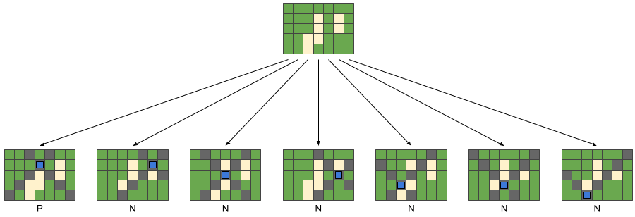
Since only one of those states is a P-position, the answer to Case #1 is 1.
Test Set 1
For this test set, since we only have at most $$$10$$$ spots available for new attractions, we can simply use brute force search with the above recursion rules to decide whether a given game state is $$$N$$$-position or $$$P$$$-position.
The game tree size and the state-space complexity of this game both have size $$$O(S!)$$$, where $$$S$$$ represents the number of spots available to build an attraction on the initial game state. For each state, in addition to the recursion for next states, we also need $$$O(\min(\mathbf{R},\mathbf{C}))$$$ time to mark the new advertisement signs on the board. Therefore, the brute force search solution to this problem has time complexity $$$O(S! \times \min(\mathbf{R},\mathbf{C}))$$$.
In this brute force search, using dynamic programming to store every seen state won't help decrease the time complexity because the size of the dynamic programming table we will end up with is still up to $$$O(S!)$$$.
Test Set 2
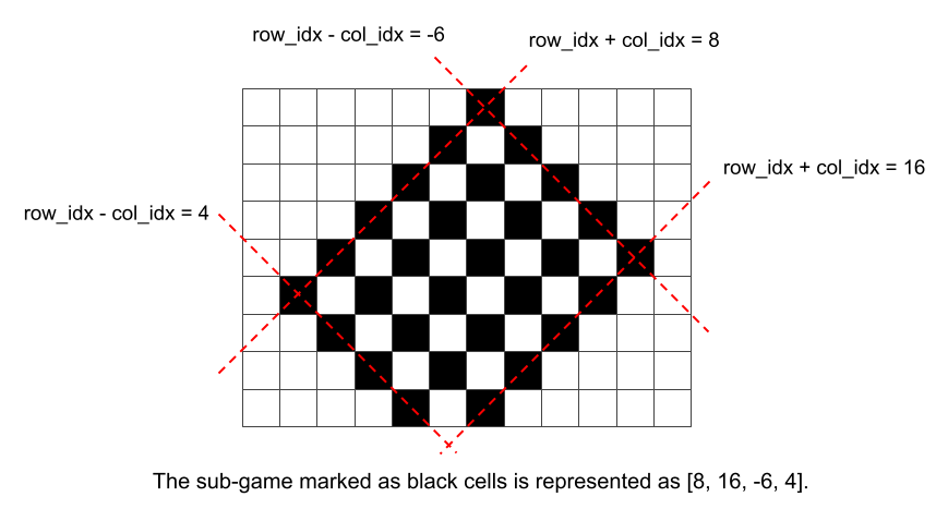
Since the sign builders always extend in the diagonal direction like chess bishops, the cells on the game board can actually be seen as two independent parts: the black cells and the white cells in a chessboard shown below.
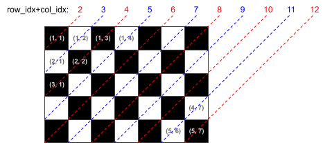
Formally, from each attraction, only cells that have the same row_idx+col_idx
parity can be affected. See the chess board above, the black cells have even
row_idx+col_idx, while the white cells have odd row_idx+col_idx.
Furthermore, since the sign builders only extend until they reach an occupied cell, the areas that were previously divided by other extending signs are also independent. And the independent areas with no available spot to build can simply be ignored.
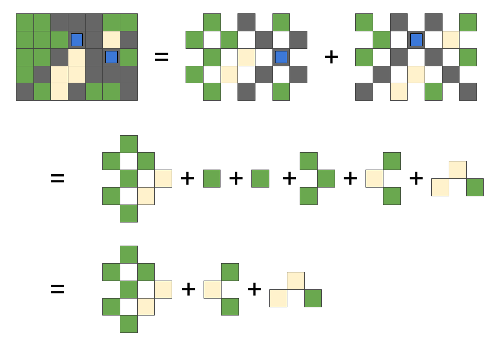
For example, the top left is a board with $$$2$$$ attractions built on $$$(2,4)$$$ and $$$(3,6)$$$. This board is equal to $$$6$$$ independent "sub-games" shown above. And from observation, we can see only $$$3$$$ of them have available spots, and each of them will be completely occupied in one move. Therefore, there are exactly $$$3$$$ moves remaining to finish the game no matter how the players play. So we can easily figure out that this example is an $$$N$$$-position (the next player wins).
To formalize the calculation steps we demonstrated, we need the Sprague-Grundy theorem. According to the Sprague-Grundy theorem, if we have an impartial game in which the players take turns to play exactly one move and the player who cannot move loses, we can assign each game state a value (called the $$$SG$$$-value). Each game-state's $$$SG$$$-value only depends on the $$$SG$$$-value of the game-states we can reach with exactly one move.
Specifically, for any game state $$$s$$$, we have:
If a state $$$s$$$ is split into several independent sub-games $$$\{q_1, q_2, \dots, q_k\}$$$, the $$$SG$$$-value of $$$s$$$ can be calculated as $$$$SG(s)=SG(\{q_1, q_2, \dots, q_k\})=SG(q_1) \oplus SG(q_2) \oplus \cdots \oplus SG(q_k),$$$$ where $$$\oplus$$$ is the binary xor function.
Finally, if $$$SG(s)=0$$$, then $$$s$$$ is a $$$P$$$-position; otherwise $$$s$$$ is an $$$N$$$-position. So the goal of this problem is to find out how many spots on the given initial game state the player can build an attraction on and turn the game state into $$$SG$$$-value = 0.
The recursive function to calculate the $$$SG$$$-value of a given sub-game can be implemented as:
-
a sub-game can be represented by a tuple
[row_idx_plus_col_idx_begin, row_idx_plus_col_idx_end, row_idx_minus_col_idx_begin, row_idx_minus_col_idx_end], like the example shown above, - for each available spots in this range, put an attraction on it and calculate the new $$$SG$$$-value. Then the $$$SG$$$-value of this sub-game is calculated by applying $$$\text{mex}$$$ to them. And
-
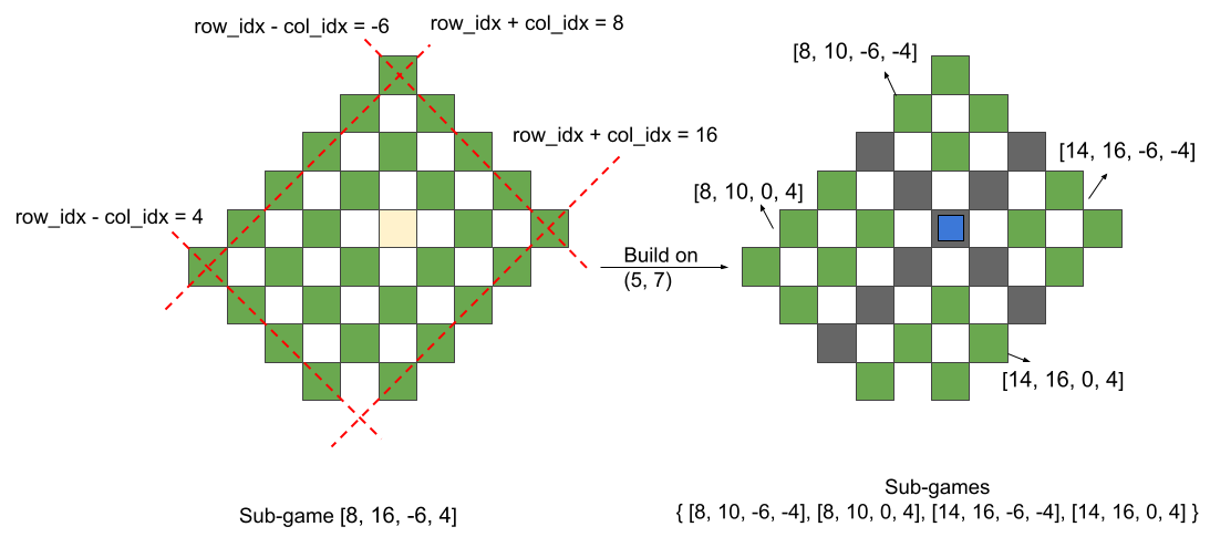
when an attraction is put on a spot
[row_idx, col_idx], the current sub-game[row_idx_plus_col_idx_begin, row_idx_plus_col_idx_end, row_idx_minus_col_idx_begin, row_idx_minus_col_idx_end]is divided into four new sub-games[row_idx_plus_col_idx_begin, row_idx + col_idx - 2 , row_idx_minus_col_idx_begin, row_idx - col_idx - 2 ],[row_idx_plus_col_idx_begin, row_idx + col_idx - 2 , row_idx - col_idx + 2 , row_idx_minus_col_idx_end],[row_idx + col_idx + 2 , row_idx_plus_col_idx_end, row_idx_minus_col_idx_begin, row_idx - col_idx - 2 ],[row_idx + col_idx + 2 , row_idx_plus_col_idx_end, row_idx - col_idx + 2 , row_idx_minus_col_idx_end],
Now we know how to use the Sprague-Grundy theorem. Take Sample Case #1 as an example, what will happen if Izabella puts her attraction at third row and sixth column?
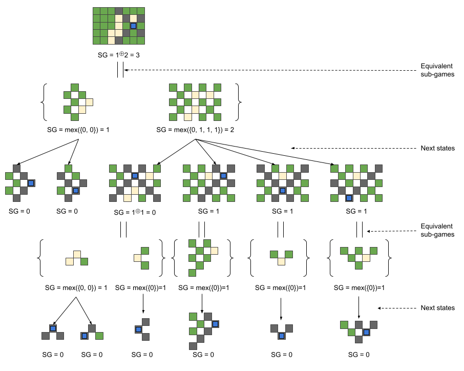
We can see that putting the first attraction on this cell will give an $$$SG$$$-value of 3. This means that Olga will having a winning move from this position, which is not good for Izabella!
Note that we can use dynamic programming to store the $$$SG$$$-value of each seen sub-game. In this way, the state-space complexity of this search is $$$O(\mathbf{R}^2 \times \mathbf{C}^2)$$$. And when calculating the $$$SG$$$-value of each sub-game, we need to visit all $$$O(S)$$$ available spots in it to enumerate the next states. When adding an attraction, we don't need to actually mark those $$$O(\min(\mathbf{R},\mathbf{C}))$$$ advertisement signs, we only need to use constant time to split the sub-games and calculate XOR from their results. Therefore, the total time complexity of this solution is $$$O(S \times \mathbf{R}^2 \times \mathbf{C}^2)$$$. And since $$$S$$$ is $$$O(\mathbf{R}\times\mathbf{C})$$$, the time complexity can also be written as $$$O(\mathbf{R}^3\times \mathbf{C}^3)$$$.