Google Code Jam Archive — Round 3 2021 problems
Overview
Round 3 started with Build-A-Pair, a punny but not puny problem that required the right greedy approach in order to save lots of casework, and the time that comes with it. As in most recent Round 3s, there was a significant step up in difficulty going into the second problem. Square Free, a problem a lot more appropriate this year than the past one, required a combination of graph theory, a clever ad-hoc insight, and iterative improvements to solve.
Of course, the last two problems are where the key to getting to the finals was hidden. Fence Design was the always scary geometry problem. It could be solved in many different ways. Knowing your geometry theorems and algorithms could definitely put you on the right path, but all of them required the right customization to solve the problem. Finally, the path to solve Binary Search Game was hardly monotonic. The right model and usual game theory could get you some points, but some advanced arithmetic manipulation was needed for the full amount.
There were a flurry of submissions for Build-A-Pair early in the contest, but it took several minutes until someone managed to get the full score. Square Free was also solved shortly afterwards, but it took 54 minutes for the first full solution to Binary Search Game to arrive, and over 75 minutes for Fence Design to get solved.
Because there were a lot of partially correct solutions to the last two problems, the scoreboard jumped around a lot. Gennady.Korotkevich was the only one to get to a full 100 points for solid first place. xll114514 and Um_nik rounded out the top 3 by getting 81 points (all but Test Set 2 of Fence Design), and 12 other coders also managed to get to 81. In the end, a total of 683 people submitted something, with 601 of them getting points. The unofficial cutoff to get to the finals is 55 points and low enough penalty, which corresponds to solving the first two problems and Test Set 1 of the last two. Congratulations to all contestants for tackling such a hard set!
In about two months, our finalists will face off in the World Finals! The Finals will take place virtually for a second year in a row. Finalist or not, everyone who advanced to Round 3 will be able to remember their accomplishment by wearing the coveted Code Jam 2021 shirt! We will be sharing lots of video content during the finals, so please tune in to share the excitement with us!
Cast
Build a Pair: Written by Pablo Heiber. Prepared by Artem Iglikov.
Square Free: Written by Ian Tullis. Prepared by Darcy Best and Timothy Buzzelli.
Fence Design: Written by Pablo Heiber. Prepared by Pablo Heiber and Timothy Buzzelli.
Binary Search Game: Written by Yui Hosaka. Prepared by Petr Mitrichev.
Solutions and other problem preparation and review by Andy Huang, Artem Iglikov, Darcy Best, Deepika Naryani, Hannah Angara, Joe Simons, John Dethridge, Kevin Tran, Liang Bai, Max Ward, Md Mahbubul Hasan, Mekhrubon Turaev, Mohamed Yosri Ahmed, Nafis Sadique, Pablo Heiber, Petr Mitrichev, Sadia Atique, Swapnil Gupta, Timothy Buzzelli, Vaibhav Tulsyan, and Yui Hosaka.
Analysis authors:
- Build a Pair: Artem Iglikov.
- Square Free: Darcy Best.
- Fence Design: Pablo Heiber.
- Binary Search Game: Kevin Tran.
A. Build-A-Pair
Problem
You want to build a pair of positive integers. To do that, you are given a list of decimal digits to use. You must use every digit in the list exactly once, but you get to choose which ones to use for the first integer and which ones to use for the second integer. You also get to choose the order of the digits within each integer, except you cannot put a zero as the most significant (leftmost) digit in either integer. Note that you cannot choose just a zero for one integer either, because it would not be positive.
For example, you could be given the list $$$[1, 0, 2, 0, 4, 3]$$$. Two of the valid pairs you can build are $$$(200, 143)$$$ and $$$(3, 12400)$$$. The following pairs, on the other hand, are not valid:
- $$$(0102, 34)$$$: has a leading zero.
- $$$(0, 12340)$$$: has a non-positive integer.
- $$$(10, 243)$$$ and $$$(12300, 47)$$$: the list of digits in each of these pairs is not exactly equal to the given list of digits.
Given the list of digits to use, what is the minimum absolute difference between the two built integers that can be achieved?
Input
The first line of the input gives the number of test cases, $$$\mathbf{T}$$$. $$$\mathbf{T}$$$ lines follow. Each line describes a test case with a single string of digits $$$\mathbf{D}$$$. Each character of $$$\mathbf{D}$$$ is a digit you must use.
Output
For each test case, output one line containing Case #$$$x$$$: $$$y$$$,
where $$$x$$$ is the test case number (starting from $$$1$$$) and $$$y$$$
is the minimum possible absolute difference between the two integers built from $$$\mathbf{D}$$$
according to the rules above.
Limits
Time limit: 5 seconds.
Memory limit: 1 GB.
$$$1 \le \mathbf{T} \le 100$$$.
Each character of $$$\mathbf{D}$$$ is a decimal digit.
At least two characters of $$$\mathbf{D}$$$ are not 0.
Test Set 1 (Visible Verdict)
$$$2 \le$$$ the length of $$$\mathbf{D} \le 8$$$.
Test Set 2 (Visible Verdict)
$$$2 \le$$$ the length of $$$\mathbf{D} \le 36$$$.
Sample
4
1234
0011
07080
0899
Case #1: 7
Case #2: 0
Case #3: 620
Case #4: 1
The optimal pair of integers to build are $$$31$$$ and $$$24$$$ for Sample Case #1, $$$10$$$ and $$$10$$$ for Sample Case #2, $$$700$$$ and $$$80$$$ for Sample Case #3, and $$$89$$$ and $$$90$$$ for Sample Case #4.
B. Square Free
Problem
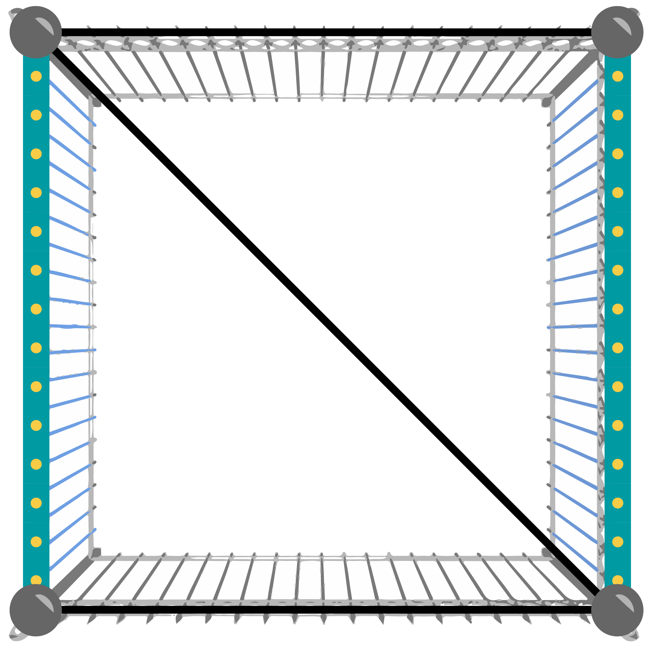
We have a matrix of square cells with $$$\mathbf{R}$$$ rows and $$$\mathbf{C}$$$ columns. We need to draw a diagonal in each cell. Exactly one of two possible diagonals must be drawn in each cell: the forward slash diagonal, which connects the bottom-left and the top-right corners of the cell, or the backslash diagonal, which connects the top-left and the bottom-right corners of the cell.
For each row and column, we want to draw a specific number of diagonals of each type. Also, after all the diagonals are drawn, the matrix should be square free. That is, there should be no squares formed using the diagonals we added.
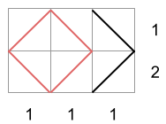
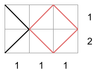
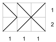
For example, suppose we have a matrix with $$$4$$$ rows and $$$4$$$ columns. The number next to each row is the exact number of forward slash diagonals there must be in that row. The number below each column is the exact number of forward slash diagonals there must be in that column.
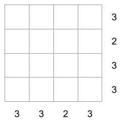
There are multiple ways to fill the matrix respecting those per-row and per-column amounts. Below we depict three possibilities:
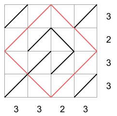
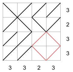
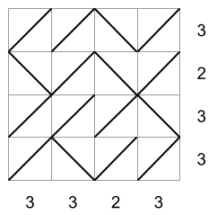
The first two matrices are not square free, while the third matrix is. In the first matrix, there is a square of side-length $$$2$$$ diagonals with its vertices in the middle of each side of the matrix. In the second matrix, there is a square of side-length $$$1$$$ diagonal drawn in the bottom-right corner. In the third matrix, there is no square. The third matrix would then be a valid drawing according to all the rules.
Given the size of the matrix and the exact number of forward slash diagonals that must be drawn in each row and column, produce any square free matrix that satisfies the row and column constraints, or say that one does not exist.
Input
The first line of the input gives the number of test cases, $$$\mathbf{T}$$$. $$$\mathbf{T}$$$ test cases follow. Each test case consists of exactly three lines. The first line of a test case contains $$$\mathbf{R}$$$ and $$$\mathbf{C}$$$, the number of rows and columns of the matrix. The second line of a test case contains $$$\mathbf{R}$$$ integers $$$\mathbf{S_1}, \mathbf{S_2}, \dots, \mathbf{S_R}$$$. $$$\mathbf{S_i}$$$ is the exact number of forward slash diagonals that must be drawn in the $$$i$$$-th row from the top. The third line of a test case contains $$$\mathbf{C}$$$ integers $$$\mathbf{D_1}, \mathbf{D_2}, \dots, \mathbf{D_C}$$$. $$$\mathbf{D_i}$$$ is the exact number of forward slash diagonals that must be drawn in the $$$i$$$-th column from the left.
Output
For each test case, output one line containing Case #$$$x$$$: $$$y$$$,
where $$$x$$$ is the test case number (starting from 1) and $$$y$$$ is
IMPOSSIBLE if there is no filled matrix that follows all rules
and POSSIBLE otherwise. If you output POSSIBLE,
output $$$\mathbf{R}$$$ more lines with $$$\mathbf{C}$$$ characters each.
The $$$j$$$-th character of the $$$i$$$-th of these lines
must be / if the diagonal drawn in the $$$i$$$-th row from the top
and $$$j$$$-th column from the left in your proposed matrix is a forward slash
diagonal, and \ otherwise. Your proposed matrix must be valid according to
all rules.
Limits
Time limit: 15 seconds.
Memory limit: 1 GB.
$$$1 \le \mathbf{T} \le 100$$$.
$$$0 \le \mathbf{S_i} \le \mathbf{C}$$$, for all $$$i$$$.
$$$0 \le \mathbf{D_i} \le \mathbf{R}$$$, for all $$$i$$$.
Test Set 1 (Visible Verdict)
$$$2 \le \mathbf{R} \le 6$$$.
$$$2 \le \mathbf{C} \le 6$$$.
Test Set 2 (Hidden Verdict)
$$$2 \le \mathbf{R} \le 20$$$.
$$$2 \le \mathbf{C} \le 20$$$.
Sample
4
4 4
3 2 3 3
3 3 2 3
2 3
1 1
1 1 1
2 3
1 2
1 1 1
3 3
2 0 2
2 0 2
Case #1: POSSIBLE
//\/
\/\/
///\
/\//
Case #2: IMPOSSIBLE
Case #3: POSSIBLE
\\/
//\
Case #4: POSSIBLE
/\/
\\\
/\/
Sample Case #1 is the one explained above.
In Sample Case #2, there must be a total of $$$2$$$ forward slash diagonals according to the sum of the row totals, but a total of $$$3$$$ according to the sum of the column totals. It is therefore impossible to follow all rules.
In Sample Case #3 the only matrices that follow the row and column totals are the following:
Since the first two contain a square, the third one is the only valid output for this case.
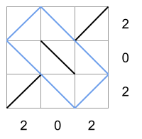
In Sample Case #4 there is only one way to fill the matrix that follows the row and column totals, shown in the picture below. Note that it produces a single rectangle, shown in blue in the picture. But, since that rectangle is not a square, the matrix is square free.
C. Fence Design
Problem
You are hired as a temporary employee of the Fence Construction Company and have been tasked with finishing the design of the fencing for a field. Each fence must run in a straight line between two poles. Each pole occupies a single point and the location of each pole is fixed. No three poles are collinear. Fences cannot intersect each other, except possibly at their endpoints (the poles).
The design was started by someone else, but they quit the project after adding exactly two fences. You need to finish their design. To impress your bosses and clients, you want the design to have as many fences as possible, regardless of their lengths.
Given the positions of the poles and the already-built fences, please find a way to add as many fences as possible such that no pair of fences (new or existing) intersect each other, except possibly at their endpoints (the poles).
Input
The first line of the input gives the number of test cases, $$$\mathbf{T}$$$. $$$\mathbf{T}$$$ test cases follow. Each test case starts with a single line containing an integer $$$\mathbf{N}$$$, indicating the number of poles. Then, $$$\mathbf{N}$$$ lines follow. The $$$i$$$-th of these lines contains two integers $$$\mathbf{X_i}$$$ and $$$\mathbf{Y_i}$$$, representing the X and Y coordinates of the $$$i$$$-th pole's position. The last two lines for each test case represent the two existing fences. These two lines contain two integers each: $$$\mathbf{P_k}$$$ and $$$\mathbf{Q_k}$$$, representing that the $$$k$$$-th existing fence runs between the $$$\mathbf{P_k}$$$-th and the $$$\mathbf{Q_k}$$$-th pole (poles are numbered starting from $$$1$$$).
Output
For each test case, output one line containing Case #$$$x$$$: $$$y$$$,
where $$$x$$$ is the test case number (starting from 1) and $$$y$$$ is the maximum
number of fences that can be added to the design (not including the existing ones).
Then, output $$$y$$$ more lines. Each line must contain two distinct integers
$$$i$$$ and $$$j$$$ (both between $$$1$$$ and $$$\mathbf{N}$$$, inclusive),
representing a different fence that connects the $$$i$$$-th and $$$j$$$-th poles.
No pair of the $$$y+2$$$ fences (the existing fences as well as the ones
you have added) may overlap, except possibly at their endpoints.
Limits
Memory limit: 1 GB.
$$$1 \le \mathbf{T} \le 50$$$.
$$$-10^9 \le \mathbf{X_i} \le 10^9$$$, for all $$$i$$$.
$$$-10^9 \le \mathbf{Y_i} \le 10^9$$$, for all $$$i$$$.
$$$(\mathbf{X_i}, \mathbf{Y_i}) \neq (\mathbf{X_j}, \mathbf{Y_j})$$$, for all $$$i \neq j$$$.
$$$1 \le \mathbf{P_k} \lt \mathbf{Q_k} \le \mathbf{N}$$$, for all $$$k$$$.
The existing fences do not intersect, except possibly at their endpoints.
No three poles are collinear.
Test Set 1 (Visible Verdict)
Time limit: 60 seconds.
$$$4 \le \mathbf{N} \le 100$$$.
Test Set 2 (Hidden Verdict)
Time limit: 90 seconds.
$$$4 \le \mathbf{N} \le 10^5$$$.
Sample
2
4
0 0
0 1
1 1
1 0
1 2
3 4
5
0 0
0 1
1 1
1 0
2 3
1 2
3 5
Case #1: 3
1 4
2 3
4 2
Case #2: 6
5 4
2 4
5 2
1 4
4 3
3 2
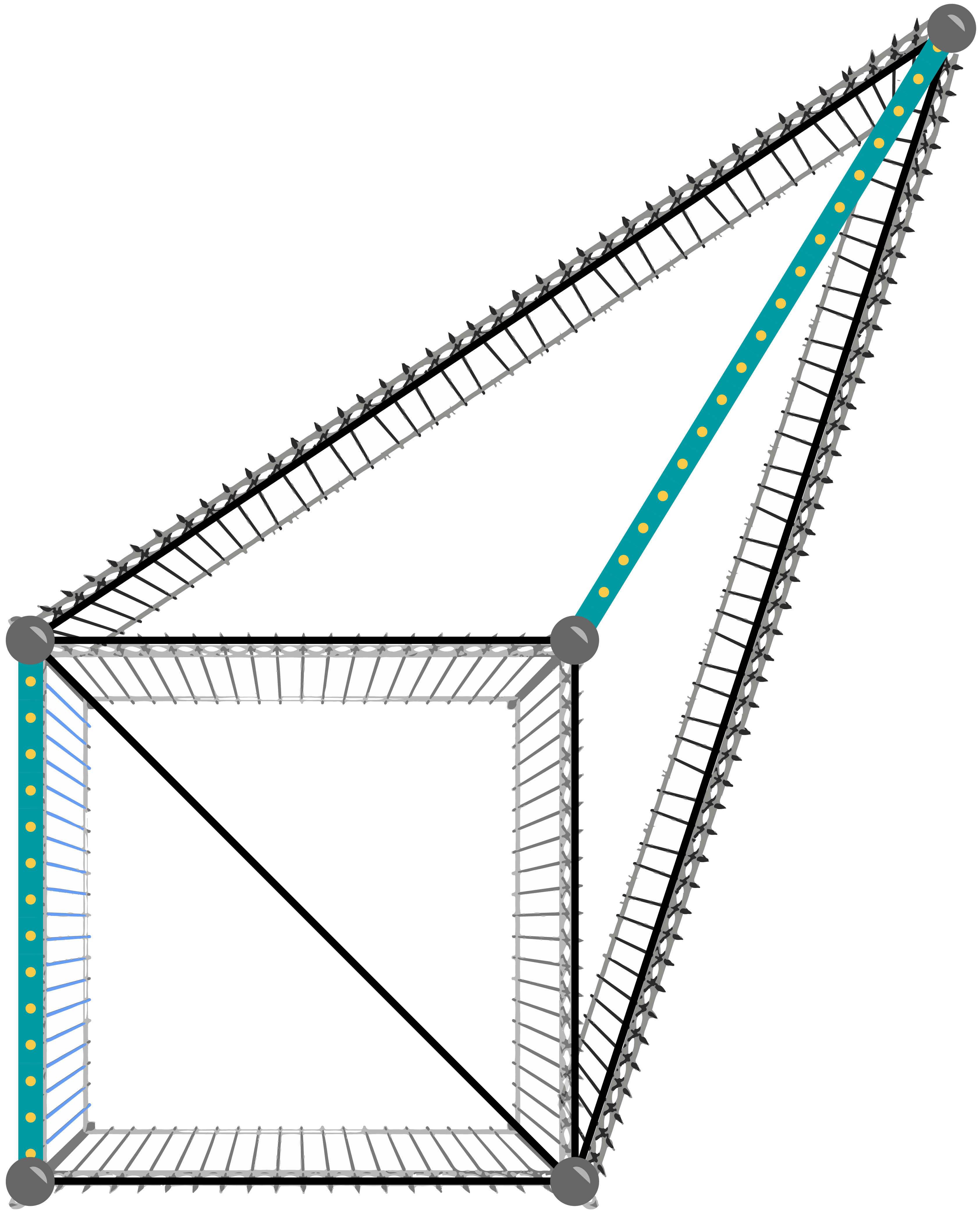
The following pictures show the poles and fences in the given samples. The fences with the wider blue line on them are the existing ones, and the rest show the way of adding a maximum number of fences shown in the sample output.
D. Binary Search Game
Problem
Alice and Bob are going to play the Binary Search game. The game is played on a board consisting of a single row of $$$2^\mathbf{L}$$$ cells. Each cell contains an integer between $$$1$$$ and $$$\mathbf{N}$$$, inclusive. There are also $$$\mathbf{N}$$$ cards numbered $$$1$$$ through $$$\mathbf{N}$$$. Before the game starts, the referee writes an integer between $$$1$$$ and $$$\mathbf{M}$$$, inclusive, on each card, in one of the $$$\mathbf{M}^\mathbf{N}$$$ ways in which that can be done. Alice and Bob know the integers in the cells and on each card before they start playing.
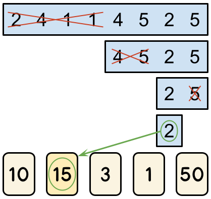
The game proceeds alternating turns, with Alice having the first turn. There are $$$\mathbf{L}$$$ turns in total, which means Alice plays $$$\lceil \mathbf{L} / 2 \rceil$$$ turns and Bob plays $$$\lfloor \mathbf{L} / 2 \rfloor$$$ turns. During a turn, a player can eliminate either the leftmost half or the rightmost half of the remaining cells. For example, let us consider a board that contains the numbers $$$[2, 4, 1, 1, 4, 5, 2, 5]$$$. In her first turn, Alice must choose to eliminate one half, leaving either $$$[2, 4, 1, 1]$$$ or $$$[4, 5, 2, 5]$$$. If she eliminates the leftmost half and leaves $$$[4, 5, 2, 5]$$$, then Bob must choose between leaving $$$[4, 5]$$$ and $$$[2, 5]$$$. If he were to leave $$$[2, 5]$$$, the game's final turn would have Alice choosing between $$$[2]$$$ and $$$[5]$$$.
When the game is over, they look at the number $$$X$$$ in the only remaining cell. The score of the game is the integer written on card number $$$X$$$. In the example above, if Alice were to eliminate $$$[5]$$$ and leave $$$[2]$$$ in her final turn, the score of the game would be the number the referee wrote on card number $$$2$$$.
Alice plays optimally to maximize the score of the game, while Bob plays optimally to minimize it. They are given a fixed board with integers $$$\mathbf{A_1}, \mathbf{A_2}, \dots \mathbf{A_{2^L}}$$$ in its cells. For maximal fairness, they will play $$$\mathbf{M}^\mathbf{N}$$$ games, and the referee will choose a different way to write integers on the cards for each one. That means that for any given way of writing integers on the cards, Alice and Bob will play exactly one game with it. Given the game parameters and the fixed board contents, please determine the sum of the scores of all those games. Since the output can be a really big number, we only ask you to output the remainder of dividing the result by the prime $$$10^9+7$$$ ($$$1000000007$$$).
Input
The first line of the input gives the number of test cases, $$$\mathbf{T}$$$. $$$\mathbf{T}$$$ test cases follow. Each test case consists of exactly two lines. The first line of each test case contains the three integers $$$\mathbf{N}$$$, $$$\mathbf{M}$$$, and $$$\mathbf{L}$$$. The second line contains $$$2^{\mathbf{L}}$$$ integers $$$\mathbf{A_1}, \mathbf{A_2}, \dots, \mathbf{A_{2^L}}$$$, where $$$\mathbf{A_i}$$$ is the integer contained in the $$$i$$$-th cell from the left of the board.
Output
For each test case, output one line containing Case #$$$x$$$: $$$y$$$,
where $$$x$$$ is the test case number (starting from $$$1$$$) and $$$y$$$ is
the sum of scores of all $$$\mathbf{M}^{\mathbf{N}}$$$ games, modulo the prime $$$10^9+7$$$ ($$$1000000007$$$).
Limits
Time limit: 30 seconds.
Memory limit: 1 GB.
$$$1 \le \mathbf{T} \le 12$$$.
$$$1 \le \mathbf{L} \le 5$$$.
$$$1 \le \mathbf{A_i} \le \mathbf{N}$$$, for all $$$i$$$.
Test Set 1 (Visible Verdict)
$$$1 \le \mathbf{N} \le 8$$$.
$$$1 \le \mathbf{M} \le 100$$$.
Test Set 2 (Hidden Verdict)
$$$1 \le \mathbf{N} \le 32$$$.
$$$1 \le \mathbf{M} \le 10^9$$$.
Sample
3
2 2 2
2 1 1 1
4 3 2
3 1 1 4
5 100 3
2 4 1 1 4 5 2 5
Case #1: 6
Case #2: 144
Case #3: 991661422
In Sample Case #1, there are $$$4$$$ ways to write the integers on the blank cards: $$$[1, 1]$$$, $$$[1, 2]$$$, $$$[2, 1]$$$, and $$$[2, 2]$$$. In the first two ways, no matter what Alice chooses in her first turn, Bob can always make the number in the last remaining cell be a $$$1$$$, and card $$$1$$$ contains a $$$1$$$, which means those two games have a score of $$$1$$$. In the last two ways, Alice can start by eliminating the leftmost half of the board, leaving $$$[1, 1]$$$ for Bob, who then has no choice but to leave $$$[1]$$$ at the end. Since card $$$1$$$ has a $$$2$$$ on it in these ways, the score of both of these games is $$$2$$$. The sum of all scores is therefore $$$1+1+2+2=6$$$.
Analysis — A. Build-A-Pair
Test Set 1
With the total number of digits up to 8 we can iterate through all possible pairs of numbers we can construct from these digits and choose the optimal one. One way to do this is to iterate through all possible permutations of the given digits and then split every permutation into two in all possible ways as if it were a string. For every such a split we can construct the numbers and calculate the answer. Be careful though, as numbers should not start with 0, every split where 0 is the first digit in a number is not valid.
If we denote the length of $$$D$$$ as $$$N$$$, then this takes $$$O(N! \times N^2)$$$ time.
Test Set 2
First we can calculate the lengths of each resulting number. These should be as close as possible, which means in case $$$N$$$ is even, each number must have exactly $$$N / 2$$$ digits, and if $$$N$$$ is odd, then the larger number must have $$$\lceil N / 2\rceil$$$ digits and the smaller number must have $$$\lfloor N / 2 \rfloor$$$ digits.
Further we will refer to the larger number as $$$A$$$ and to the smaller number as $$$B$$$.
Now, let's deal with the case when $$$N$$$ is odd. In such a case, we can iterate through all non-zero digits and try them as the first digit of $$$A$$$ and $$$B$$$. Now we would want to make $$$A$$$ as small as possible (as it is already larger than $$$B$$$), and $$$B$$$ as large as possible. Luckily, these two goals are complementary: we can use the $$$\lfloor N / 2 \rfloor$$$ smallest remaining digits to construct the rest of $$$A$$$ (just take them in non-decreasing order), and use the rest to construct $$$B$$$ (by taking them in non-increasing order). Notice that choosing the leading digits greedily is also possible, but care must be taken to not choose zero. This way of simply trying everything only takes $$$O(b^2 \times N)$$$ time anyway, where $$$b$$$ is the base ($$$10$$$), which is fast enough for the limits of the problem.
The case when $$$N$$$ is even is trickier, as just choosing the first digits does not give us a unique way to construct the rest of $$$A$$$ and $$$B$$$, because there is no guarantee that $$$A$$$ will be larger. However, we can use similar technique as part of the solution.
Note that if we have a prefix of length $$$i$$$ $$$A_1 A_2 \dots A_i$$$ of $$$A$$$ and prefix $$$B_1 B_2 \dots B_i$$$ of $$$B$$$, we can guarantee that $$$A$$$ will be larger than $$$B$$$ no matter what digits we use further if and only if there is a $$$k \le i$$$ such that $$$A_j = B_j$$$ for all $$$1 \le j \lt k$$$ and $$$A_k > B_k$$$. This gives us the following algorithm: choose all possible ways to construct $$$A_1 A_2 \dots A_{k-1}$$$ and $$$B_1 B_2 \dots B_{k-1}$$$, then iterate through all possible $$$A_k$$$ and $$$B_k$$$, then construct the rest of $$$A$$$ and $$$B$$$ so that the former is as small as possible and the latter is as large as possible, using the same technique as above. For each of these possibilities, update the answer with the difference between the constructed numbers. Note, as before, that we need to make sure that the numbers we construct do not start with 0.
The time complexity of such an algorithm is $$$O(2^{N / 2})$$$ for selecting $$$A_1 A_2 \dots A_{k-1}$$$ and $$$B_1 B_2 \dots B_{k-1}$$$ (these are pairs of equal digits, so we cannot have more than $$$N / 2$$$ of them, and the order among them is irrelevant, as long as we do not start with zero), $$$O(b^2)$$$ for selecting $$$A_k$$$ and $$$B_k$$$, and $$$O(N)$$$ for constructing the numbers once we got the prefixes. Overall this gives us $$$O(2^{N / 2} \times b^2 \times N$$$, which is really fast in practice with a good implementation.
The algorithm can be optimized further, but it is not required for the given constraints. There are ways to use the fact that number of digits is limited to reduce $$$2^{N/2}$$$ to something with $$$b$$$ (the base) instead of $$$N$$$ in the exponent. There is also a way to greedily solve the full problem in linear time. Moreover, if the input and output are given in run-length encoding, it can be solved in linear time in that encoding of the input, which is $$$O(\log N)$$$.
Analysis — B. Square Free
Test Set 1
In general, we will build all grids with the correct row and column sums,
then check each one to see if there are squares in them.
In Test Set 1, the size of the input is at most $$$6 \times 6$$$. This means that
there are $$$2^{36}$$$ different possible grids, which is too many to generate, so we
must make use of the row sum constraints. We do this by building the grid one cell at a time. As
you fill in each cell, ensure that corresponding row and column sums are still possible.
For example, if the row sum should be 3, but there are already 3 /s in this
row, you cannot put another /. Similarly, if the desired row sum is 3,
but there are already $$$\mathbf{R}-3$$$ \s in the row, you cannot put another
\. Once we are done filling out the grid,
we check if there are any squares in the grid that we have made. If there are no squares,
we are done! Otherwise, we move on to the next possible grid. If we finish searching
all possible grids and we have not found any, then it is impossible.
Are we sure this is fast enough? Each row either needs 0, 1, 2, 3, 4, 5, or 6
/s in it. There are $$$\binom{6}{0} = 1$$$ choices with 0 /s,
$$$\binom{6}{1} = 6$$$ choices with 1 /s,
$$$\binom{6}{2} = 15$$$ choices with 2 /s,
$$$\binom{6}{3} = 20$$$ choices with 3 /s,
$$$\binom{6}{4} = 15$$$ choices with 4 /s,
$$$\binom{6}{5} = 6$$$ choices with 5 /s, and
$$$\binom{6}{6} = 1$$$ choices with 6 /s.
Thus, each row has at most 20 different valid choices. So this algorithm will explore
at most $$$20^6$$$ different grid. In practice, we will get nowhere near this bound.
In particular, there is at most one valid row for the bottom row (since we must
satisfy the column sum constraints). This alone reduces the search space to
at most $$$20^5$$$, but this, too, is an overestimate since there will be
a lot of pruning throughout the search.
Checking for squares can be done in several ways. The easiest is to iterate over
all possible places that the top-most row of the square can be (and which consecutive
columns the /\ are in). Then, for each possible size of square (1, 2, 3),
just check the corresponding grid entries on the four sides of the square.
Test Set 2
The bounds for Test Set 2 are much too large to exhaustively search all grids, so we will need an insight. We call a grid that satisfies the row and column constraints a configuration. First, let's discuss how to find some configuration (it may or may not be square free). To do this, we will set this up as a graph and run maximum flow on it. There are $$$\mathbf{R}$$$ vertices that represent the rows and $$$\mathbf{C}$$$ vertices that represent the columns. We will put an edge with capacity 1 between every pair of (row, column) vertices. We will then connect the $$$i$$$-th row vertex to a super-row vertex with capacity $$$\mathbf{S_i}$$$ and connect the $$$i$$$-th column vertex to a super-column vertex with capacity $$$\mathbf{D_i}$$$.
We now run flow through the network using the super-row vertex as the source and
the super-column vertex as the sink. If the network is saturated (that is, every edge
leaving the source has flow = capacity), then we have a solution. If there is flow
in the edge between row $$$r$$$ and column $$$c$$$, then the corresponding entry in the
grid is a /, otherwise it is a \. If the flow is not saturated,
then it is impossible to make a grid with the appropriate row and column sums. We leave
a formal proof of the bijection between configurations and valid flows on the described
network as an exercise.
At this point, we have some configuration, but it may have squares in it. We will discuss three different ways to produce a grid that is square free.
Lexicographically Smallest Configuration
In this solution, we notice that the
lexicographically smallest
configuration (treating \ as smaller than / reading in
row-major order)
is square-free! At first this is not obvious. However, think about two rows
($$$r_i \lt r_j$$$) and two columns ($$$c_k \lt c_{\ell}$$$). If
$$$(r_i, c_k) = /, (r_i, c_{\ell}) = \backslash, (r_j, c_k) = \backslash, (r_j, c_{\ell}) = /$$$,
then this grid is not the lexicographically smallest configuration. Why? Because we can
swap all four of those without breaking the row or column constraints, while giving us a
smaller configuration
($$$(r_i, c_k) = \backslash, (r_i, c_{\ell}) = /,
(r_j, c_k) = /, (r_j, c_{\ell}) = \backslash$$$).
This means that a lexicographically smallest configuration has no squares in the grid, because
the top-most row of a square must contain /\ in the same columns in which
the bottom-most row of the square has \/.
How do we find the lexicographically smallest configuration? There are two ways:
(1) give the edge between row $$$r$$$ and column $$$c$$$ a cost of
$$$2^{r-1+(c-1)\mathbf{R}}$$$ and run
minimum-cost maximum-flow.
This will guaranteed find the lexicographically smallest, but the edge-costs will be
huge (up to $$$2^{\mathbf{RC}-1}$$$).
(2) We will run maximum flow iteratively. Say we have run maximum flow. Go through the
edges in row-major order of their corresponding cell. If there is no flow going through an
edge, then it is a
\. Great! This is the smallest this can be, so remove this edge from the graph
to lock that in. If there is flow going through the edge, then we "unpush" the flow from that
edge (decrease the flow from the sink to the column vertex to the row vertex to the source by 1)
and temporarily change that edge's capacity to 0. We then run flow again. If the flow
is still saturated, then we know there exists a configuration where this entry in the
grid is a \, so we can permanently remove this edge from the graph.
If it is not saturated, then we must put that edge back into the graph, and this entry
is forced to be a /.
Complexity-wise, the first run of maximum flow takes $$$O( (\mathbf{RC})^2 )$$$ time. Then, for each flow we run, we must only push one unit of flow through, which only takes a single augmenting path, so $$$O(\mathbf{RC})$$$ time per edge. Thus, in total, this takes $$$O( (\mathbf{RC})^2 )$$$ time. Note that you can also fully re-run maximum flow for each edge instead of only pushing one unit of flow with a sufficiently optimized flow implementation.
Minimum-Cost Maximum-Flow
In the Lexicographically Smallest Configuration solution, we described how you can use minimum-cost maximum flow to solve this problem with exponential edge costs. Here, we will solve the problem using only polynomial sized edge costs. This solution makes use of the same idea as the previous one: we want to avoid $$$(r_i, c_k) = /, (r_i, c_{\ell}) = \backslash, (r_j, c_k) = \backslash, (r_j, c_{\ell}) = /$$$, but other than that, we do not need a lexicographically smallest configuration. If we set the edge cost between row $$$r$$$ and column $$$c$$$ to be $$$r \times c$$$, then we will not get this configuration, since swapping all of these symbols does not affect the row/column sums and strictly decreases the total cost. The total cost is reduced by $$$i \times k + j \times \ell$$$ and increased by $$$i \times \ell + j \times k$$$, which is a net decrease of $$$(i - j)(k - \ell) > 0$$$ since $$$i \lt j$$$ and $$$k \lt \ell$$$.
Flip-Flop!
Another solution is to simply find some configuration, then check it for squares. If there
are no squares, then we are done! If there is a square, consider the top-most and bottom-most
row in the square. We will swap the top /\ with the bottom \/.
This does not affect the row/column sums. In doing this, we have broken the current square, but
may have created another square. We continue breaking squares until we do not find
any. This process must eventually finish since at each swap, we are always making our grid
lexicographically smaller. You can never do more than $$$O( (\mathbf{RC})^2 )$$$ swaps of this form.
Common Mistake
Be careful! Just because the sum of the $$$\mathbf{S_i}$$$s is equal to the sum of the $$$\mathbf{D_i}$$$s does not mean that a configuration exists! One example is the following input, where those sums coincide, yet there are no grids that meet all the per-row and per-column requirements.
4 6
2 0 6 6
4 2 2 2 2 2
Analysis — C. Fence Design
This problem asks us to find a triangulation of the given set of points that uses two particular edges. Many of the arguments that follow are referenced in the linked article, so you can use it as an introduction.
The first step to solve this problem is to notice some properties of the finished job. Let $$$P$$$ be the input set of poles and $$$F$$$ be a maximum set of fences with endpoints in $$$P$$$ that do not intersect other than at endpoints.
1. The fences that are the edges of the
convex hull of $$$P$$$ are in $$$F$$$.
Proof: By definition, the edges of the convex hull do not intersect with any other possible
fence. Therefore, they can be added to any set of fences that do not contain them without
generating any invalid intersections, so any maximum set contains them all.
2. The size of $$$F$$$ is at most $$$3\mathbf{N} - 3 - c$$$ where $$$c$$$ is the size of the convex hull of
$$$P$$$.
Proof: Consider the graph where poles are nodes and fences in $$$F$$$ are the edges. The graph is
planar, so the generalized form of
Euler's formula applies. The formula states that $$$\mathbf{N} + A = K + |F|$$$, where $$$A$$$
is the number of internal areas (not counting the outside) and $$$K$$$ the
number of connected components of the graph.
Notice that each edge on the convex hull is adjacent to exactly one internal area, and other edges are adjacent to at most two internal areas. Therefore, the sum of the number of sides of all internal areas is at least $$$3A$$$ and that is counting each convex hull edge once and each other edge at most twice, so $$$3A \le c + 2(|F| - c) = 2|F| - c$$$, which means $$$A \le (2|F| - c) / 3$$$. Replacing that in Euler's formula we obtain $$$\mathbf{N} + (2|F| - c) / 3 \ge K + |F|$$$. It follows that $$$3\mathbf{N} + 2|F| - c \ge 3K + 3|F|$$$, and then $$$3\mathbf{N} - c - 3K \ge |F|$$$. Since $$$K \ge 1$$$, we obtain $$$|F| \le 3\mathbf{N} - 3 - c$$$.
3. The size of $$$F$$$ is at least $$$3N - 3 - c$$$.
Proof: By induction. The base case is when all points in $$$P$$$ are on the convex hull.
For that case, consider a set of all edges in
the convex hull of $$$P$$$ plus any
triangulation
of $$$P$$$. This set has exactly $$$2N - 3$$$ edges, which is equal to $$$3\mathbf{N} - 3 - c$$$ when
$$$\mathbf{N} = c$$$, proving that there exists a set of at least that size without any invalid
intersections.
If there exists a point $$$p$$$ not on the convex hull of $$$P$$$, consider an optimal set of edges for $$$P - {p}$$$, which by inductive hypotheses has size $$$3(\mathbf{N} - 1) - 3 - c$$$. Because $$$|F| = 3(\mathbf{N} - 1) - c - 3$$$, and $$$3(\mathbf{N} - 1) - c - 3K \ge |F|$$$ from (2), $$$K$$$, the number of connected components, must be exactly one. Similarly, every internal area must be a triangle, with all edges in the convex hull being adjacent to one of them and all edges not in the convex hull being adjacent to two of them. By definition, $$$p$$$ is not on the convex hull. By the fact that there are no collinear triples, $$$p$$$ is not in an existing edge. Thus, $$$p$$$ is strictly contained in one of these triangles. Therefore, we can add edges from $$$p$$$ to each of the $$$3$$$ vertices of the triangle that contains $$$p$$$ to get a solution for our problem of size $$$3(\mathbf{N} - 1) - 3 - c + 3 = 3\mathbf{N} - 3 - c$$$.
From (2) and (3) above we know the exact number of fences we need to build (given the size of the convex hull of the set of poles). Moreover, we know that such an answer contains the convex hull of $$$P$$$ and every internal area delimited by fences in the output is a triangle. We can use this to devise algorithms to generate optimal sets.
Test Set 1
There are many possible solutions for Test Set 1. For example, the procedure in the proof of point (3) above shows how to solve the problem with no pre-placed fences. There are ad-hoc ways to get around the problems with pre-placed fences, but they take a lot of work, and there is something simpler.
The proofs above show that any maximal set of fences is also maximum (notice that we only used maximality in our reasoning). Therefore, we can simply add fences to a set as long as they do not intersect with any previously added fence. This algorithm can accommodate pre-placed fences quite easily: simply start with them. There are $$$O(\mathbf{N}^2)$$$ potential fences to consider, and for each one we need to check whether it intersects any of the fences we already have. Since the solution overall is of size $$$O(\mathbf{N})$$$ this means checking $$$O(\mathbf{N}^3)$$$ intersections. Checking a pair of line segments to see if they intersect can be done in constant time, which means this algorithm takes $$$O(\mathbf{N}^3)$$$ time overall.
Test Set 2
As in Test Set 1, there are lots of algorithms that solve this problem without considering the pre-placed fences, but only some of them are easy enough to adapt to them. For example, the procedure from the proof of (3) can be implemented efficiently: if the order in which we process points is randomized and we keep the current triangles in a tree-like structure to perform the search for a triangle efficiently, we can get an expected $$$O(\mathbf{N} \log \mathbf{N})$$$ time complexity. This leads to an algorithm similar to the incremental algorithm to compute a Delauney triangulation.
Another option is to modify the Graham Scan algorithm to efficiently find the convex hull to keep not only a convex hull of the visited points, but also all the triangles for the points inside it.
Unfortunately, while the algorithms above can work with a lot of ad-hoc code to accommodate the pre-placed fences, they become really cumbersome. Below we present some better alternatives.
Let $$$x$$$ be the intersection of both lines that are the infinite extension of a pre-placed fence. Since the fences don't intersect, $$$x$$$ can occur on one of them, but not on both. Let us call any pre-placed fence that does not contain $$$x$$$ $$$f_1$$$, and the other fence $$$f_2$$$. By their definitions, all of $$$f_2$$$ is on the same side of the line that extends $$$f_1$$$. We can recognize which fence can be $$$f_1$$$ by comparing whether the orientation of the two endpoints of a potential $$$f_1$$$ and each endpoint of $$$f_2$$$ is the same (that is, checking whether both endpoints of the candidate $$$f_2$$$ lie on the same side of the line that goes through $$$f_1$$$).
Sweep-line
We can solve the problem without pre-placed fences with a sweep-line that considers the points in order of x-coordinate and maintains a convex hull of all the already seen points, as in the monotone chain convex hull algorithm. When considering a new point $$$p$$$, we simply connect it to all points from the already-seen set that do not cause intersections from $$$p$$$. Notice that those points are a continuous range of the right side of the convex hull of the already-seen set. Therefore, we can find those points efficiently with ternary searches on its right side.
To accommodate pre-placed fences, we first rotate the plane to make $$$f_2$$$ vertical (possibly scaling everything to use only integers) and then run the sweep line algorithm only on points that are on the same side of the line that goes through $$$f_1$$$ as $$$f_2$$$ (including both endpoints of $$$f_2$$$ and neither endpoint of $$$f_1$$$). Since $$$f_2$$$ is now vertical, it will be included by the algorithm in the set when its second endpoint is processed. After that, we rotate everything again to make $$$f_1$$$ vertical, and start the algorithm from the set and convex hull we already have (the endpoints of $$$f_1$$$ will be the first two points that are processed in this second pass). As before, $$$f_1$$$ will be added naturally by the algorithm.
Notice the accommodation of the pre-placed fences only requires linear time work, so the overall algorithm, just as the version without pre-placed fences, requires $$$O(\mathbf{N} \log \mathbf{N})$$$ time overall.
Divide and conquer
This divide and conquer algorithm also has a correlate to computing the convex hull. The idea is simple: divide the set of points with a line that goes through $$$2$$$ points, compute the result of each side (both of which include those $$$2$$$ points), and then combine.
Let us call the two recursive results $$$P$$$ and $$$Q$$$. The convex hulls of both are convex polygons with a shared side. Then, we keep two current poles $$$p$$$ and $$$q$$$. Initially, both $$$p$$$ and $$$q$$$ are on the same endpoint of the shared side. Both move away from that shared side: $$$p$$$ through consecutive vertices of $$$P$$$ and $$$q$$$ through consecutive vertices of $$$Q$$$. Initially we move them both together. After that, let $$$p_0$$$ and $$$q_0$$$ be the previous pole where $$$p$$$ and $$$q$$$ were, respectively, and $$$p_1$$$ and $$$q_1$$$ be the next value for each (that is, $$$p_0p$$$ and $$$pp_1$$$ are adjacent sides of the convex hull of $$$P$$$ and $$$q_0q$$$ and $$$qq_1$$$ are adjacent sides of the convex hull of $$$Q$$$). Then,
- If $$$p_1q$$$ does not intersect $$$p_0p$$$, we set $$$p = p_1$$$.
- If $$$q_1p$$$ does not intersect $$$q_0q$$$, we set $$$q = q_1$$$.
- Otherwise, we stop.
To divide evenly, we can pick any point $$$x$$$, sort the other points by angle, and pick the median as $$$y$$$, dividing by the line that goes through $$$x$$$ and $$$y$$$. Alternatively, we can pick points randomly. On average, the split of points would be about even (as we did in the proposed solution for Juggle Struggle: Part 1).
The work done to combine takes linear time and the work done to split takes either $$$O(\mathbf{N} \log \mathbf{N})$$$ time for the sorting version or linear time for the randomized version. Using the Master theorem we can then see that using the randomized version, the overall algorithm takes $$$O(\mathbf{N} \log \mathbf{N})$$$ time, and using the sorting version, the overall running time is $$$O(\mathbf{N} \log^2 \mathbf{N})$$$.
Analysis — D. Binary Search Game
Test Set 1
Let $$$f(k)$$$ be the number of ways in which the game ends with a score $$$\geq k$$$. Then, the number of ways in which the game ends with a score of exactly $$$k$$$ is $$$f(k) - f(k+1)$$$. Therefore, the answer is $$$$\begin{align} \sum_{k=1}^{\mathbf{M}} k(f(k) - f(k+1)) &= \sum_{k=1}^{\mathbf{M}} k f(k) - \sum_{k=1}^{\mathbf{M}} k f(k+1) \\ &= \sum_{k=1}^{\mathbf{M}} kf(k) - \sum_{k=2}^{\mathbf{M}+1} (k-1)f(k) \\ &= f(1) - \mathbf{M} f(\mathbf{M}+1) + \sum_{k=2}^{\mathbf{M}} (k - (k-1)) f(k) \\ &= \sum_{k=1}^{\mathbf{M}} f(k). \end{align}$$$$ Notice in the last step that $$$f(\mathbf{M}+1) = 0$$$ by definition.
Let us now focus on calculating $$$f(k)$$$. For each card, we only care about whether its value is $$$\geq k$$$ or not. Let $$$S$$$ be a fixed subset of cards which have value $$$\geq k$$$ (we will go through all $$$2^\mathbf{N}$$$ such subsets). We can assign a score of $$$0$$$ (for cards outside of $$$S$$$) or $$$1$$$ (for cards in $$$S$$$) to each consecutive subsequence of cells on the board that can be presented to players, in increasing order of length. Notice that only subsequences of cells whose length is a power of $$$2$$$ and who are "aligned" can be presented to a player. That is, sequences containing cells of the form $$$i2^j+1,i2^j+2,\dots,i2^j+2^j$$$ for each $$$j$$$ between $$$0$$$ and $$$\mathbf{L}$$$, inclusive, and each $$$i$$$ between $$$0$$$ and $$$2^{\mathbf{L}-j}-1$$$, inclusive. There are $$$2^\mathbf{L} + 2^{\mathbf{L}-1} + \cdots + 2 + 1 = 2^{\mathbf{L}+1} - 1$$$ valid combinations to go through. If we know the score for sequences of shorter lengths, we can decide the score for a sequence by checking whose turn it is (it is Alice's turn if and only if $$$j$$$ and $$$\mathbf{L}$$$ have the same parity) and picking either the maximum or the minimum score of its two halves. If the score assigned by this to the full sequence is $$$0$$$, then there is no way to finish with a score $$$\geq k$$$ with combination $$$S$$$. Otherwise, we need to compute the number of ways in which this can happen. This is simply the number of original card values that yield $$$S$$$, which is $$$(\mathbf{M}-k+1)^t (k-1)^{\mathbf{N}-t}$$$ where $$$t$$$ is the number of cards that are $$$\geq k$$$ in $$$S$$$.
Overall, this solution takes $$$O(\mathbf{M} \times 2^\mathbf{N} \times 2^\mathbf{L})$$$ time, which is fast enough to pass Test Set 1.
Test Set 2
Note that the expression $$$(\mathbf{M}-k+1)^t (k-1)^{\mathbf{N}-t}$$$ from the previous solution, if we consider $$$k$$$ the only variable, expands into a polynomial of degree at most $$$\mathbf{N}$$$. Consequently $$$f(k)$$$ is also a polynomial in $$$k$$$ of degree at most $$$\mathbf{N}$$$ (as it is the sum of such polynomials).
If $$$f(k)$$$ is a polynomial of degree at most $$$\mathbf{N}$$$, then $$$g(x) = \sum_{k=1}^{x} f(k)$$$ is a polynomial in $$$x$$$ of degree at most $$$\mathbf{N}+1$$$. This is a consequence of Faulhaber's formula.
Thus, the polynomial $$$g(x)$$$ can be fully determined by evaluating it at $$$\mathbf{N} + 2$$$ different points, say $$$g(0), g(1), \ldots, g(\mathbf{N}+1)$$$. We can evaluate those values in the same way as Test Set 1 and then use interpolation to find $$$g(\mathbf{M})$$$.
This yields an algorithm that takes time $$$O(\mathbf{N} \times 2^\mathbf{N} \times 2^\mathbf{L})$$$ to evaluate $$$\mathbf{N} + 2$$$ points of $$$f(k)$$$, plus the time complexity of evaluating $$$g(\mathbf{M})$$$ using interpolation. The latter can be done by evaluating the Lagrange polynomial in a straightforward way in $$$O(\mathbf{N}^2)$$$, and there are faster methods too, but this does not impact the overall runtime.
To speed up the calculation of $$$g(0), g(1), \ldots, g(\mathbf{N}+1)$$$, we find a way to reduce the $$$2^\mathbf{N}$$$ factor. Note that if a card's index appears only once (or not at all) in the board, we can do without fixing its value in advance (as being $$$\geq k$$$ or not). We can fix the values that are repeated in the board and then run the greedy algorithm but instead of scores $$$0$$$ and $$$1$$$ we compute, for each subsequence, the number of ways that it can be made $$$1$$$ by assigning the values of cards whose indices are not repeated in the board. The decisions can still be made greedily, but instead of doing all the combinatorics at the end, we do them at each decision point.
With this optimization, we only need to run the greedy algorithm $$$2^X$$$ times per each value of $$$g$$$ that we need, where $$$X$$$ is the number of cards whose indices appear more than once in the board. There can be at most $$$2^{\mathbf{L}-1}$$$ of those cards, so we have reduced the time complexity of the first step to $$$O(\mathbf{N} \times 2^{2^{\mathbf{L}-1}} \times 2^\mathbf{L})$$$. This is finally enough to pass Test Set 2.