Google Code Jam Archive — Virtual World Finals 2020 problems

Test Set 1

A translation of the problem statement is that we wish to find the minimum cost maximum flow on a directed tree. The rest points can be represented by nodes, and the ski slopes can be represented by edges. A commonly used algorithm to solve minimum cost maximum flow problems is successive shortest paths. In the case of our directed tree, a simplified successive shortest paths approach can be applied.

Observe that we can add skiers greedily. Of all the nodes that can be reached from the top of the mountain (the root of the tree), we should always send a skier to a node with a minimum cost path using only edges that still have capacity remaining. Since we are working with a tree, there is only one path from the root to each node. With this in mind, we can find the path costs to all the nodes using any tree traversal from the root while calculating the cost to each node as the cost of its parent (which we calculated first) plus the cost of the edge connecting them. Then, we can sort the nodes by their path cost in ascending order. We should always use the first node in the list that still has some capacity along its path.

Let us maintain the number of skiers sent through each edge. We can work through our sorted list of nodes in order. We check if the current node in the list still has some capacity by checking the edges in the path, and either update the capacities if we can push another skier, or move on to the next node in the list if we cannot. Doing this for a single skier takes O(N) time. We know we will keep using the same path until some edge reaches capacity, so we can compute the minimum capacity left in the path with a linear pass over it, and simulate sending that many skiers at once. Each such a step takes O(N) time overall, and since we have to try up to O(N) possible destinations, the overall algorithm takes O(N²) time, which is efficient enough to solve Test Set 1.

Test Set 2

For the large input, we need to do more. We can use a heavy light decomposition of the tree to manage the remaining capacities of the edges in the tree. The decomposition will need to support updates and queries on paths from the root to an internal node. The updates involve subtracting an amount from the capacity of each edge. The queries involve finding the minimum capacity of all the edges on a path.

A heavy light decomposition breaks a tree up into a collection of disjoint paths such that the number of decomposition paths from any node to the root is at most O(log N). If we keep a segment tree for each decomposition path, then we can support both the query and update operations in O(log² N). Note that the segment tree we use must support lazy range updates. This improves the running time of each step of the algorithm for Test Set 2 to take only O(log² N) time instead of O(N) time. This makes the algorithm run in O(N log² N) time in total, which is sufficient to solve the Test Set 2.

As is the case in many problems about games, this problem revolves around evaluating a given state of the game and deciding whether it is winning or losing. The problem defines mistakes as transitions from winning to losing states, so once we have determined the type of each state, we can easily count up the mistakes.

Test Set 1

In all zero-sum finite two person games with no ties, the basic framework to decide whether a state is winning is the same. Let us call a state A-winning (or equivalently, B-losing) if player A can ensure a win from it, or B-winning/A-losing otherwise. For a given state, if the game is over, check the winning condition. Otherwise, if it is player X's turn, try every possible play. If any of them leads to an X-winning state, then the current state is also X-winning. Otherwise, the current state is X-losing. We can implement this as a recursive function, but given that there can be O(N²) possible plays on any given turn, this will only work quickly enough for small values of N.

We can see immediately that there can be a lot of repeated work in that recursive evaluation. For example, consider a state S and another state S' such that S' is the result of making P plays on S. Since there are P! ways to make those plays, state S' potentially needs to be evaluated P! times to evaluate S once. Memoizing the function or turning it into a dynamic programming implementation would thus save a lot of recursive calls.

In addition, there are many states that can be evaluated without the need for a recursive call. Some simple cases include states in which there already are two adjacent and consecutive tiles placed (the "already won" condition for player A). We can prune the recursive calls tree by simply returning those states as A-winning. We can prune it further: if there is a play that creates such a pair during A's turn (the "can win immediately" condition), we just do that instead of trying all possible plays for A. We can also restrict B to only try plays that do not leave a known A-winning condition. There are ways to prune the tree further, some of which we explore in the Test Set 2 section below.

We can pass Test Set 1 either with a combination of simple pruning and memoization/dynamic programming, or a lot of pruning.

Test Set 2

The number of possible states in Test Set 2 is just too big to even fit in memory, even after careful pruning. However, pruning enough can help us find sets of equivalent states, that is, groups of states that we can prove have the same winner. By doing that, we can dramatically reduce the number of memoized states.

Consider only A's turns first. We have already mentioned the "already won" and "can win immediately" conditions above. On top of those, we can notice that if there is some set of three unplayed tiles available with three consecutive numbers, and there is some block of three consecutive cells available, A can win by playing the middle number in the middle cell (we call this the "can win in 2 moves" condition). Whatever B plays next, A's following turn will fulfill either the "already won" condition or the "can win immediately" condition.

The conditions above allow us to find some states which are definitely A-winning. Notice that in any other state where it is A's turn, it's impossible for any of the already-placed tiles to end the game as part of an adjacent and consecutive pair. Therefore, they could be replaced by "unavailable" cells without a specific number on them. So, the remaining cells can be represented as the multiset of sizes of the groups of consecutive cells that are left; call it L_C. The exact locations of those groups on the board are not relevant to the final outcome. Since each tile can only form adjacent and consecutive pairs with other leftover tiles, we can similarly represent the remaining tiles with a multiset of lengths of consecutive runs of tiles; call it L_T. For example, the state

7 2 6 _ _ 3 _ 4 _ _ 5

has the leftover tiles 1, 8, 9, 10, 11, so its leftover cells can be represented by the multiset L_C = {1, 2, 2} and its leftover tiles by the multiset L_T = {1, 4}.

In addition, since the "can win in 2 moves" condition has already been checked, we know that at least one of L_C and L_T does not contain any integer greater than or equal to 3. To simplify the algorithm, notice that the game in which we swap tile numbers and cell numbers is equivalent (because the winning condition is symmetric). Therefore, states with L_C and L_T swapped are equivalent. We can therefore assume it is always L_C that has only integers 1 and 2.

After this compression, the number of states is dramatically reduced. Notice that because we know that there are no three consecutive leftover numbers, at least N/3 numbers have been played already. That means that the sum of the integers in both L_C and L_T (which is the same for both multisets) is at most 2×N/3. Therefore, the total number of possible multisets L_T under those conditions is bounded by the sum of partitions(K) for every K between 0 and 2×N/3, which is partitions(2×N/3+1). Given such an L_T multiset, the number of possible multisets L_C of only 1s and 2s such that the sum of L_C and L_T is the same is bounded by N/3 (which is the maximum number of 2s). So, the number of states is no greater than (N/3)×partitions(2×N/3+1), which is a fairly small number for the given limits for N. Moreover, we need only one memoization or dynamic programming table for all test cases.

There are multiple sufficiently fast ways to implement the second player's turns (which are the slowest ones), and there are further restrictions that can be placed on plays to optimize our strategy even more. Some of those options result in an algorithm whose complexity makes it clear that it runs within the time limit. Some other options have a theoretical complexity that is either too large or hard to estimate tightly enough to be convinced it's fast enough. Fortunately, it's possible to compute the recursive function for all possible states without reading any data, and be sure that it runs in time before submitting.

The Test Set 3 that wasn't

We considered having a third test set for this problem requiring a polynomial solution. We progressively found solutions taking O(N³) time, O(N²) time and even one requiring only O(N log N) time. We ultimately decided against adding the test set because the possibility of solving it by guessing the right theorem without proof was a significant concern. The benefit of the extra challenge without making contestants have to read a full extra statement is of course a significant benefit, but it was dampened by our estimation that the likelihood of it being solved legitimately was small. If we had made it worth a small number of points, it would not have been worth the relative effort to solve it. If we had made it worth a lot, though, that would have diminished the value of the work needed for our favorite part of the problem, which is solving Test Set 2.

If you are up to try an extra challenge without spoilers, stop here. If you want some hints on how those solutions go, read ahead!

The first theorem further compresses the states considered in the Test Set 2 solution on A's turns. Consider a state that is not under the "already won", "can win immediately" or "can win in 2 moves" conditions represented by some multisets L_C and L_T, where only L_T can contain integers greater than 2. That state is A-winning if and only if the state represented by multisets L_C and L'_T is A-winning, where L'_T is obtained from L_T by replacing each integer X in L_T with floor(X / 2) copies of a 2 and a 1 if X is odd. This reduces the number of states of the dynamic programming to O(N³), and we can process each of those states in constant time because there is only a bounded number of effectively different plays to make.

If we pursue that line of reasoning further, we can find that we can check A-winningness with a small number of cases. Let L_Ci be the number of times i is in L_C, and L_Ti be the number of times i is in L_T. Because we already assumed that L_C had no integers greater than 2, L_Ci = 0 for all i ≥ 3. Let K = L_C1+2×L_C2 = sum of i×L_Ti over all i be the number of turns left and Z = (L_T2+L_T3) + 2×(L_T4+L_T5) + 3×(L_T6+L_T7) + ... be the number of times 2 appears in L'_T as described in the previous paragraph. Then, the second theorem we can prove is that:

• If K = 2, then the state is A-winning if and only if L_C2 = L_T2 = 1.
• If K > 2, then the state is A-winning if and only if K is odd and 2×(L_C2+Z) > K.

From the need to avoid the "already won", "can win immediately" and "can win in 2 moves" conditions, it is possible to reduce the number of plays on B's turn to a set of a bounded number of options that always contains a winning move if there is one. This, together with the fact that the conditions above can be checked in constant time, yields an algorithm that decides for any state whether it is winning or losing in O(N) time, making the overall process of a test case take O(N²) time. With some technical effort, we can represent the board in a way that we can update and use in O(log N) time to check all the necessary conditions, yielding an algorithm that requires only O(N log N) time to process a full test case.

The proofs for the theorems on the paragraphs above are left as an exercise to the reader. As a hint, it is easier to prove the second more general theorem, which is already nicely framed, and then obtain the first theorem as a corollary.

The main task in this problem is to count how many ways there are to pick a permutation and a pair of numbers from the list such that their (possibly truncated) sum falls within the given interval. This is the numerator of a fraction representing the desired probability. The number of total picks (our denominator) is simply 16! × N × (N - 1) / 2. Then, we can use a known algorithm (like dividing numerator and denominator by the greatest common divisor) to reduce the fraction to the desired form. In the rest of the analysis, we focus only on calculating the non-reduced numerator.

One common denominator among all solutions for all test sets is that the actual values of the digits in the list do not matter. Once we fix a pair of numbers X and Y from the list, only the "digit structure" of the pair (X, Y) matters. The digit structure of a pair of numbers is a unique way to see their coupling as digits. We define it as the lexicographically smallest pair (P[X], P[Y]) across all possible digit permutations P, where P[X] is the result of replacing each digit of X with the value assigned to it by P. Notice that digit structures have length 2D.

The total number of digit structures grows rapidly when D increases, but depends only on D, which has small limits. The total number is 15 for D=2, 203 for D=3, 4140 for D=4, and 115975 for D=5.

Test Set 1

In Test Set 1, the number of different digit structures is really small. In addition, for a fixed structure, we only care about the values assigned by the chosen permutation to up to 2D digits. For each digit structure with d unique digits, we can compute the value of the truncated sum for a valid assignment of those d digits, noting that there are (16 - d)! ways to generate each assignment.

The number of valid assignments can be somewhat large at 16! / 10! or about 6 million for 6 different digits, but there is only one digit structure within Test Set 1 that has that many different digits. There are a handful that have 5, for which there are around half a million assignments each, and most structures have 4 or fewer different digits, which have fewer than 50 thousand different assignments each. Moreover, this computation only depends on D and not on the rest of the input, so we have to do it only once for each possible structure for D=2 and D=3.

Given the precomputation above, we can iterate over the pairs of integers from the list, compute their digit structures, and use two binary searches to see how many of the numbers in the list are in range. Then, we compute the number of different digits in the structure d and multiply the total by (16 - d)!, which gives us the number of sums in range that can be produced for the given pair. Summing that result over all possible pairs gives us the answer we need.

Test Set 2

The precomputation above can be slow in Test Set 2. Not only do we have 4140 additional digit structures to process, but most importantly, a few of those have 7 and 8 unique digits. Each additional digit means an order of magnitude extra possible assignments. There are several ways to handle this, and we need only a few of the tricks below to make it work.

The first issue is that the lists we need to store are now too long to fit in memory. Since there are only up to 16⁴ different results, many of those results would be repeated, so we can compress them based on those repetitions. This is still tough to pull off, so the best thing to do is to just not store the full list. We know we only care about how many items on the list are in range for up to T different ranges. So, we can read all cases before starting the computation, split the full range of sum results at every A and B that we read into up to 2T+1 minimal ranges, and then compress together all numbers that are within the same range. This definitely fits in memory.

We can also choose to not memoize between different test cases, and treat them one at a time. If we do that, we have a fixed A and B, so there is no need for lists, just a counter. We can either treat each pair of numbers individually as well (speeding up the process of assignments — see below) or try to memoize digit structures if any are repeated within the same test case. It is possible that almost every pair has a different digit structure, of course, but there are few digit structures with the maximum number of unique digits. This means the memoization reduces the total runtime in what was our previously worst case, and the new worst case (all different structures) is not as bad because many of those structures will have fewer different digits.

We can reduce the number of digit structures further by realizing that digit structures like (011, 022) and (012, 021) are equivalent, in the sense that for any assignment, their sum is the same: both are 11 × (P[2] + P[3]) + 100 × P[0], where 11 and 100 are in base 16. This only works in conjunction with some form of memoization.

Once we have either a range [A, B] or a small list of ranges fixed at the moment of processing the assignments, we can use it to do some pruning. Suppose we assign values to the digits in most significant positions first. When we have done a partial assignment, we can compute or estimate a range of possible values that the sum may have when we finish. As more highly significant digits get assigned, that range shrinks. If that range is completely inside our target range (or one of our target ranges) we can stop and know that all further assignments work, counting them using a simple multiplication. If the range is completely outside of the target range (or all target ranges), we can also stop and count nothing further.

As mentioned above, we need only some of the optimizations above to manage to pass Test Set 2. Of course, the more of them we find and implement, the more confident we can be about the speed of our solution.

Test Set 3

To simplify the problem, we can use a common technique when dealing with counting numbers in closed intervals [A, B]. We write a function f(U) that only calculates the value for closed intervals [0, U-1]. Then, the result for an interval [A, B] is f(B + 1) - f(A). In this case, we can use this to take care of the overflow as well, by simply ignoring the overflow and counting the number of hits in the interval [A, B] plus the number of hits in the interval [16^D + A, 16^D + B], which are the only possible sums whose truncation would yield a result in [A, B]. After we write our function f, this translates to a result of f(B + 1) + f(16^D + B + 1) - f(A) - f(16^D + A). We focus now on calculating f(U), that is, the number of picks of a permutation and a pair of numbers that yield a (non-truncated) sum of strictly less than U.

Both the number of possible values a sum can have and the possible number of pairs are small (for computers). We can use an asymmetric "meet in the middle" approach to take advantage of both those facts. We do this in a similar way as what we did for Test Set 1 and possibly for Test Set 2, by keeping a count on each digit structure, and then iterating over the pairs of numbers from the list to see how much we have to use each of those counts.

First, let's consider all the ways to add up to something less than U. Let us fix the first number to have a value of x, so the second number can have any value less than U-x. A number y is less than U-x if and only if it has a smaller digit than U-x at the first position at which they differ. We can represent this set of ys by saying they are all the ys that start with the first i digits of U-x, then continue with a digit d smaller than the (i+1)-th digit of U-x, and any remaining digits can be any digit.

For example, if U=2345 and x=1122, then U-x=1223 and y can be of the form 0***, 10**, 11**, 120*, 121*, 1220, 1221, 1222, where * represents any digit.

For each pair of an x and a prefix for y, we can represent all the pairs of numbers from the list that match by matching that with a digit structure that allows for *s at the end. In this way, a pair of numbers from the list X and Y can be mapped to x and y by a permutation if they have the same digit structure, disregarding the actual digit values. To represent this, we normalize the digit structure as we did before: no digit appears for the first time before another smaller digit. Therefore, a structure like x=1122 and y=10** is represented as x=0011 and y=02**. As before, the number of permutations that can match a pair of numbers to this digit structure is (16 - d)!, where d is the number of unique digits that appear in the structure.

Notice that different values of x can yield the same structure. For example, x=1133 yields U-x=1212, and for y=10** the structure is the same as for x=1122 and y=10**.

For each digit structure of 2D total digits that have between 0 and D-1 asterisks at the right end, we count the number of permutations that make its parts add up to something less than U.

We now process the pairs of numbers from the list. For each pair, we build its normalized digit structure as before, and add the count for that digit structure to our running total. We also add the count of the structures that result in replacing up to D-1 rightmost digits with *s.

We can express the complexity of this algorithm in terms of the base B, the number of digits of each number D, and N, the size of the list of numbers. The first stage iterates through up to O(B^D) possible values for x, and for each one, considers up to O(B×D) digit structures for y. If factorials up to B are precomputed, and we store the results in a hash table or an array with a clever hashing for digit structures that keeps hashes unique and small, this requires only constant time per pair, so O(B^D+1×D) time overall. The second stage requires processing up to O(D) digit structures per pair, so it takes O(N²×D) time in total. The sum of both stages gives us the overall time to compute f, which is O(B^D+1×D + N²×D). Since we need only a constant number of calls to f, that is also the overall time complexity of our algorithm.

Another solution is to to use all of our Test Set 2 tricks in an efficient way. Consider especially the last one: when considering the pair of i-th most significant digits, only the pairs whose sum is close to either that value at A or that value at B produce a range of possible sums for the pair that is neither fully inside [A, B] nor fully outside of it. That means that for the i-th digits, there are only a linear number of pairs of digits that can be assigned at that position that would make the process not stop immediately, instead of a quadratic number. This shrinks the number of assignments to approximately the square root of its previous value, behaving more as exponential on D than as an exponential on 2D. This gives us a time complexity comparable to that of the other solution presented above. While the overall time complexity is still higher, these two solutions can perform pretty similarly for the limits we have: the bound on the number of assignments is actually smaller than B^D because it behaves more like B! / (B - D)!. Those savings, plus those from not needing extra D terms, make up for the fact that the backtracking solution's time complexity has a term with behavior similar to B^D and a term with behavior similar to N² multiplied together instead of added.

Notice that the basic insights of both solutions are closely related. The pruning provides such a large speedup for the same reason that we can use the "meet in the middle" approach based on digit structures.

Test Set 1

In this problem, we are given a circle, a collection of points around the perimeter of the circle, and the attachment values for each of those points (L_i). We want the top K pairs of points that maximizes the Euclidean distance between the points plus their attachment values. For Test Set 1, we know that the point values are picked randomly. We will need to use this property somehow. We also know that K=1, so we are looking for the top pair of points.

Imagine considering the points around the circle in the clockwise order. Let us say that we are at a point p. Also, without loss of generality, let us only consider points that are at most 180 degrees clockwise from p. That is, we only consider half of the circle starting at p. If we find the maximum pairing (maximum distance plus attachment values) for every possible p, the maximum over all of those pairs will be the answer. This is because considering each point, (and points that are up to 180 degrees clockwise from it) will consider every possible pair of points at least once.

So, we are considering all points p in the clockwise order around the circle and trying to find the maximum pairing for each of these. If we consider the possible other points we could pair with p in the counterclockwise order starting from the location 180 degrees clockwise of p (the "other side" of the circle from p), then we can observe some useful properties. Once we have considered some pairing point x, then some further counterclockwise point y will be closer to p. Thus, for y to be the maximum pairing, its attachment value must be greater than x's attachment value. So, we only need to consider points that increase in their attachment values.

We know that the attachment values are randomly selected. In a sequence of N integers randomly selected from a uniform range, we expect the running maximum to change only log N times. To see why, observe that first element has a 1/1 chance of being the new maximum, the second element has a 1/2 chance, the third element has a 1/3 chance, and so on. This is the harmonic series. The sum of its first N terms is bounded by O(log N). Thus, we expect to see only O(log N) changes of maximum. This means the explained solution has an expected time complexity of O(N log N), which should be fast enough to pass. The worst case among all possible inputs takes O(N²) time. However, as we showed, this is extremely unlikely with random attachment values.

Now, when we are considering a point x, we need an efficient way to find the first point in the counterclockwise order from x whose attachment value is greater than x. This is actually equivalent to a known problem: the next greater element problem. The twist is that our values are on a circle, so we have wraparound. One way to deal with this is to make an array of attachment values, append it to itself, and then apply a fast algorithm for the next greater element problem to the resulting array.

There are other approaches that also take O(N²) time in the worst case, because they might compare a high percentage of all pairs, but use other clever speedups like jumping to the next greater value, to have a high chance to cut the number of comparisons way down.

Test Set 2

The attachment values of points are not randomly generated in this test set, so we will need to find a different approach. Also, K=10, so we also need to find more than one pair of points. Instead of trying to find the top K pairs directly, we can find the best pairing for each point, and extend this solution to find the top K pairs overall. Let's first figure out how to find the best pairing for each point, then explain how to extend it to find the top K pairs.

We start by finding, for each input point P, which other input point Q is its best pairing. That is, we find for which other input point Q the function L_P + L_Q + distance(P, Q) is maximized.

Now consider points P not necessarily in the input. We define a value function V_P(Q) = distance(P, Q) + L_Q. Notice that if P is a point in the input, V_P(Q) + L_P is the amount of cord required to connect P and Q.

Let us approach the problem visually. Imagine moving P around the circle in the clockwise order and computing the value function V_P(Q) for all the input points Q that are up to 180 degrees clockwise of P. As we move P, how does the distance function to some other point change?

The Euclidean distance part of the distance function is equivalent to computing the length of a circular chord. That is, V_P(Q)=2×R×sin(angle(P, Q)/2)+L_Q. Notice here than the angle function is in the clockwise direction, and it's always less than or equal to 180 degrees. Consider how this function changes when P changes. That is, consider the function W_Q(P)=V_P(Q). As the domain for V_P is the Qs that are up to 180 degrees in the clockwise direction, the domain for W_Q is the Ps that are up to 180 degrees in the counterclockwise direction.

For each Q, W_Q has a constant term L_Q, and then a term that looks like half a sine wave. Notice that the graph of the function is the same for any Q, but translated: the change in angle(P, Q) translates it horizontally, and the change in L_Q translates it vertically. An example of how these graphs might look follows. Each black curve corresponds to W_Q for a different point Q.

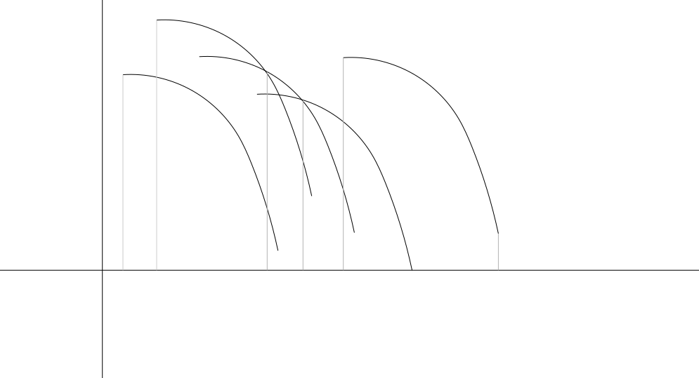
Because all of the distance functions have the same shape, we can see that W_Q has maximum values compared to all other W functions for a continuous range of points P. So, can we efficiently compute these ranges for each point? If so, we can use these ranges to find the maximum for each possible point by finding which maximum's range it falls into.

We can analyze this graph by sweeping across it from left to right—that is, increasingly along the x-axis. Since the x-axis represents points on a circle, it may be easier to visualize if we instead represent each point by its angle with respect to the positive half of the x-axis, as usual. For a fixed angle A, let us consider only the curves whose domain includes at least one point in the range [0, A] and call that set C_A. As we consider increasing values for A, at some point we consider a curve for the first time, with domain [A, B]. The curve is definitely maximum among all curves in C_A at B, because it is the only curve at that point. So, the range for which it is the maximum must end there. Since we know there is only one such range, we can binary search to find the beginning of the range.

We keep a sorted list of non-overlapping ranges as we go, and add new ranges to the end. Note that we may need to pop off some ranges from the end of the list if we find a new range that covers them completely, or shorten them if the new range covers them only partially. There can be zero or more left-most ranges where the new curve is fully under the maximum curve in that range, zero or more right-most ranges where the new curve is fully over the maximum curve in that range, and zero or exactly one range where the new curve and the curve from the range cross. We binary search within the range for the exact crossing point.

One issue we still need to deal with is that the graph is actually cyclic. It represents the distance function to points as we go around a circle. So, the distance functions we plot can "wrap around". We can deal with this via a method similar to what we used in Test Set 1: append a copy of the input to itself, and go around the input twice.

The final list of ranges can be used to get the maximum pairing for each point on the circle. For each input point P, we find the Q for which W_Q is the maximum at P. Since we only need to check input points P, we can restrict the domains of all functions and intervals discussed so far to input points without affecting the correctness. This allows us to binary search over an array of O(N) values as opposed to over a range of real numbers.

The time complexity of constructing the list of ranges is therefore O(N log N). Then, we go through the list iterating over the list of possible Ps for each Q. While a particular Q can have a long range, overall, we iterate over each input P at most once (or twice for the duplicated input). This makes the final step take linear time.

An O(N) algorithm for the above problem does exist. This is left as an exercise for the reader.

We have a way to find the best pairing for each point. How do we extend this solution to find the top K unordered pairings? It is possible that a pair in the top K is not in our list of best pairings for each point. However, we can still use our list. Consider sorting the list by the Euclidean distance plus attachment values of the pair in descending order. The first entry in the list will definitely be the top pair overall. The second top pair will either be the next entry in our list, or it will be paired with one of the points in our top pair. We can look at all pairings involving the points in our top pair, and now we know the second best pair. We can repeat this process to find the top K. In each step, the pair we choose is either the next best pair in our list that we haven't seen, or it is a pairing with a point in the previous pairs in our list. In each of these K steps, we take O(N) time. Sorting our list initially takes O(N log N) time, so our algorithm requires O(N log N + N × K) time overall, which is fast enough to pass.

The first thing we can notice is that since we replace every occurrence of a character, and at the end we count unique characters, we can regard the input S as a set. That is, multiple occurrences of the same character can be ignored, and the order of the characters is unimportant. We write "x → y" to represent the replacement of a character x by a character y. Here, and in the rest of the analysis, we use both lowercase and uppercase letters to represent variables, not actual letters that can happen in the input.

To simplify the explanations, we can represent the list of replacements as a directed graph G where nodes represent characters, and there is an edge from x to y if and only if there exists a replacement x → y in the input. Notice that each weakly connected component of G defines a problem that can be solved independently, and combining the results corresponds to adding up the number of distinct characters that can occur in the final text from each group. In particular, notice that a character c that does not appear in any replacement forms a single-node connected component, and the result for each such character is either 1 if c is in S, and 0 otherwise.

Let us define diversity as the number of unique characters in a text. Diversity of the last text is exactly what we are trying to maximize. If both x and y are in U, the diversity after performing x → y on U is 1 less than before. On the other hand, if at least one of x and y is not in U, then the diversity before and after performing x → y is the same. That is, the replacement can either cause a diversity loss of 1, or not cause any loss. We can then work on minimizing the diversity loss, and the final answer will be the original diversity minus the loss.

Test Set 1

In Test Set 1 the in-degree of each node of G is limited to at most 1. This restricts the types of weakly connected components the graph can have. If there is a node in the component with in-degree equal to 0, then the component is a directed tree and the node with in-degree equal to 0 is the root. If all nodes in the component have in-degree equal to 1, then there is a cycle (which we could find by starting at any node and following edges backwards until we see a node for the second time). Each node in the cycle only has its incoming edge coming from another node in the cycle, but it can have edges pointing out to non-cycle nodes. This means each cycle-node can be the root of a directed tree. These are the connected components of pseudoforests.

We can break down this test set by component type. Let's consider the simplest possible tree first: a simple path c₁ → c₂ → ... → c_k. If both c_k-1 and c_k are in the initial text S, then we cannot perform c_k-1 → c_k without losing diversity. No other replacement in the text can make c_k-1 or c_k disappear from the text, so they will both be present until c_k-1 → c_k is performed for the first time. In addition, after we perform c_i-1 → c_i for any i, we can immediately perform c_i-2 → c_i-1 without loss of diversity, since c_i-1 will definitely not be in the text then. Therefore, performing every replacement in the path in reverse order works optimally.

With some care, we can extend this to any tree. Consider a leaf node y that is maximally far from the root. The replacement x → y that goes into it is in a similar position as the last replacement in a path, but there could be other replacements that remove x from the text before performing x → y, which would prevent x → y from causing diversity loss. Since y is maximally far from the root, however, all other replacements that can help also lead to leaf nodes. If x and the right side of all replacements that go out of x are in S, there is no way to avoid losing diversity. However, only the first one we perform will cause diversity loss, whereas all the others can be done when x is no longer in the text, preventing further loss. We can generalize this by noticing that we can "push" characters down the tree without loss of diversity as long as there is at least one descendant node that is not in the current text. This is done by considering the path from a node x to the descendant that is not in the text y, and processing the path between x and y as described earlier.

From the previous paragraph, we can see that any edge x → y that does not go into a leaf node can be used without diversity loss. Even if there are no descendants of x in the tree that are not in the initial text S, we can process some unsalvageable leaf node first, and then we will have room to save x → y. Any edge z → w that goes into leaf nodes may be salvageable as well, as long as z has other descendants. Putting it all together, we can process the nodes in reverse topological order. At the time when we process a node x, if there is any descendant of x that is not in the current text, then we can push x down and then process all of x's outgoing edges without any diversity loss. If we process a node x and its subtree consists only of nodes representing letters currently in the text, that means that we will lose 1 diversity with the first edge going out of x that we process (it doesn't matter which one we process first), but that loss is unpreventable.

To handle cycles, consider first a component that is just a simple cycle. If there is at least one node representing a character x not in S, then we can process it similarly to paths, without diversity loss: we replace y → x, then z → y, etc, effectively shifting which characters appear on the text, but keeping diversity constant. If all characters in the cycle are in S, then the first replacement we perform will definitely lose diversity, and after that we can prevent diversity loss by using the character that disappeared as x in the process from the first case.

If a component is a cycle with one or more trees hanging from it, we can first process each tree independently. Then, each of those trees will have at least one node representing a character not in the current text: either there was such a node from the start, or it was created as part of processing the tree. So, we can push down the root of one of those trees (which is a node in the cycle) without losing diversity. Then, there will be at least one node in the cycle whose represented character is not in the text, so we can process it without diversity loss.

Test Set 2

In Test Set 2, the graph G can be anything, so we cannot do a component type case analysis like we did for Test Set 1. However, we can still make use of the idea of processing paths and pushing characters to avoid diversity loss following our first replacement.

We tackle this by morphing the problem into equivalent problems. We start with the problem of finding an order of the edges of G that uses each edge at least once while minimizing steps in which we cause diversity loss.

First, notice that once we perform x → y, we can immediately perform any other x → z without diversity loss. So, if we have a procedure that uses at least one replacement of the form x → y for each x for which there is at least one, then we can insert the remaining replacements without altering the result. That is, instead of considering having to use every edge at least once, we can simply find a way to use every node that has out-degree at least 1. Furthermore, any replacement x → y such that x is not in S can be performed at the beginning without changing anything, so we do not need to worry about using them. Notice that we are only removing the requirement of using particular edges, not the possibility. Therefore, we can make the requirements even less strict: now we only need to use every node with out-degree at least 1 that represents a character present in S.

Now that we have a problem in which we want to cover nodes, and we know from our work in Test Set 1 that we can process simple subgraphs like paths and cycles in a way that limits diversity loss, we can define a generalized version of the minimum path cover problem that is equivalent.

Given a list of paths L, let us define the weight of L as the number of paths in L minus the number of characters c not in S such that at least one path in L ends with c. That is, for each character c not in S, we can include just one path ending in c in L without adding to its weight. Let us say that a list of paths L covers G if every node in G with out-degree at least 1 that represents a character in S is present in some path in L in a place other than at the end. That is, at least one edge going out of the node was used in a path in L. We claim that the minimum weight of a cover of G is equal to the minimum number of steps that cause diversity loss in the relaxed problem.

To prove the equivalency, we first prove that if we have a valid solution to the problem that causes D diversity loss, we can find a cover that has weight at most D. Afterwards we prove that if we have a cover with weight D, we can find a solution to the problem that causes a diversity loss of at most D.

Let r₁, r₂, ..., r_n be an ordered list of replacements that satisfies the relaxed conditions of the problems and has D steps that cause diversity loss. We build a list of paths L iteratively, starting with the empty list. When considering replacement r_i = x → y:

1. If the text before and after r_i are the same, we do not change L.
2. If there is a path starting with y in L, we append x at the start of it.
3. Otherwise, we add r_i as a new path in L.

Notice that the first time we perform a replacement x → y where x is a node that we need to cover, we cannot be in case 1: the xs that were originally in S have not been replaced yet, so r_i will replace them and change the text. Cases 2 and 3 add x as a non-final part of a path. Further processing can only append things to the start of the path, so x will remain a non-final member of it. This proves that L is a cover.

Now, suppose step r_i = x → y falls into case 3 and adds a path to L that increases its weight. Because we are not in case 1, x is in the text at the time we begin to perform r_i. Since we are in case 3, there wasn't a path in L starting with y. That means that for any previous replacement of the form y → z that erased ys from the text, there was another replacement of the form w → y that that reintroduced y and caused it to no longer be a starting element of the path in L in which y → z was added. Moreover, since we are assuming this step increases L's weight, either y was in S or there is a path in L ending with v → y, which introduced y into the text. In either case, y is in the text before performing r_i, meaning that r_i causes diversity loss. Since every step that adds weight to L is a step that causes diversity loss, the weight of L is at most D.

Now let us prove that given a cover L of weight D, we can find a solution to the problem with diversity loss D. For that, we need to process paths in a manner that is not as simple as the one we used for Test Set 1. The way in which we process paths in Test Set 1 could only result in diversity loss on the first replacement made, but it also produced other changes in the text. Those changes could hurt us now that we have to process multiple paths within the same connected component.

To process a path P, we consider the status of the text U right before we start. We call a node strictly internal to a path if it is a node in the path that is neither the first nor the last node in the path. We split P into ordered subpaths P₁, P₂, ..., P_n such that the last node of P_i is the same as the first node of P_i+1 (the edges in the subpaths are a partition of the edges in P). We split in such a way that a strictly internal node of P is also a strictly internal node of the P_i where it lands if and only if the character it represents is in U. Then, we process the subpaths in reverse order P_n, then P_n-1, ..., then P₁. Within a subpath, we perform the replacements in the path's order (unlike in Test Set 1). Since the intermediate characters within a subpath do not appear in S, performing all the replacements of a subpath that starts with x and ends with y has the net effect of replacing x by y. In the case of P₁, if x is not in U, then there is no effect. After processing subpath P_i+1 that starts with x_i+1, x_i+1 is not in U, and after processing subpath P_i, x_i is not in U and x_i+1 is restored. The net effect is that processing the path in this way effectively replaces the first character of the path that is in U by the last character of the path, and doesn't change any other character.

Let L' be a sublist of L consisting of exactly one path that ends in c for each character c not in S. L - L' contains exactly D paths. We process the paths in L' first, and then the ones in L - L'. When we process a path in L', we change the text by introducing a new character to it. However, that character is not in the original S, and it is always a new one, so those changes cause no diversity loss. When processing all other paths, since the net effect is that of a single replacement, we can cause at most 1 diversity loss each time, which means at most D diversity loss overall.

Notice that if we have a path that touches a node x that represents a character in S, we can replace that node in the path with a cycle that starts and ends at x and visits its entire strongly connected component. A replacement like this one on a path in a list does not change its weight. Therefore, we can relax the condition to require covering just one node of out-degree at least 1 and with a represented character in S per strongly connected component.

We can turn this into a maximum matching problem on a bipartite graph similarly to how we solve the minimum path cover problem in directed acyclic graphs. Consider a matching M between the set of strongly connected components C (restricted to nodes representing characters in S) that need to be covered, and the set D equal to C and all remaining nodes representing characters not in S. An element c from C can be matched to an element d from D if there is a non-empty path from c to d (it cannot be matched with itself). This matching represents a "next" relationship assignment, and unmatched elements represent "ending" nodes in paths. More formally, let f(c) be the function that maps a member of C to the member of D that corresponds to the same strongly connected component. We can create a cover with weight exactly the size of the unmatched elements from C by creating a path that adds weight for each unmatched element from C, and adding paths that do not add weight for each element in D - C.

For each unmatched element c from C, add it to a new path, then append to its left its matched element M(f(c)), then M(f(M(f(c)))), etc. Then, for each matched element c in D - C, which are the characters not in S, do the same. This yields a set of paths that touches every element of C, and the ending elements are either unmatched elements from C or characters not in S which do not add weight. Notice that some unmatched elements could yield single node paths, which are paths not really considered above. However, since such a path always counts toward the weight, we can append any replacement to its end to make it not empty without increasing the weight.

Therefore, the size of the unmatched elements from C in a maximum matching of the defined relation, which we can calculate efficiently by adapting a maximum flow algorithm like Ford-Fulkerson, is equal to the minimum weight of a cover, which is what we needed to calculate.

Despite the long proofs, the algorithm is relatively straightforward to implement. The graph can be built in time linear in the size of the input, while the strongly connected components and their transitive closure, which are required to build the relation for the matching, can be found in quadratic time in the size of the alphabet A (the relation itself can have size quadratic in A, so it cannot be done faster). The maximum matching itself takes time cubic in A, because it needs to find up to A augmenting paths, each of which can take up to O(A²) time (linear in the size of the relation graph). This leads to an overall complexity of O(A³), which is fast enough for the small alphabet size of this problem. Moreover, we could use something simpler and technically slower for the strongly connected components and their transitive closure like Floyd-Warshall, simplifying the algorithm without affecting the overall running time.