Google Code Jam Archive — Round 3 2020 problems
Overview
Our first problem in Round 3, Naming Compromise, could be solved by finding the right way to extract information from a well-known algorithm. If you've been looking for a way to name a baby, and you don't mind potentially ending up with a very strange string of letters, our method might be right for you! The next problem, Thermometers, represented a big step up in difficulty, but it was tractable once you wrapped your head around the circular island presented in the problem.
The remaining two problems, Pen Testing and Recalculating, were different beasts entirely! Even a very seasoned competitive programmer might take hours to solve just one of them. Both were worth the same amount, so many contestants probably surmised that either one (plus the first two problems) could potentially serve as a pathway to the World Finals. It was a choice between creative and perhaps risky experimentation in Pen Testing, and finding the right setup and data structures for a tricky geometric situation in Recalculating.
As we expected, we got many solves of Naming Compromise early on, and solutions to Thermometers trickled in slowly but steadily. A few contestants picked off earlier test sets of Pen Testing and Recalculating. At the 1:34 mark, saketh.are became the first contestant to fully solve Pen Testing. Not long after that, at 1:45, Dlougach submitted the first full solution to Recalculating. Everything had been solved at least once, and the race was on to cobble together enough points to make the top 25!
Benq leapt to 70 points at 2:04, but our defending champion Gennady.Korotkevich sent a burst of submissions just a few minutes later, and reached an even more impressive total of 85. Surpassing that would have required solving the full set, and Gennady.Korotkevich did indeed take first in the end, followed by Benq, ecnerwala, peehs_moorhsum, and gs12117 (taking 5th with a last-minute submission!) There were various ways to advance, but it took more than the first two problems. Our contestants' overall performance was even stronger than we had predicted — you find new ways to impress us every year!
In two months, our finalists will face off in our first-ever Virtual World Finals! We will confirm the results soon and will reach out to finalists with more info. Whether or not you advanced, you'll still be able to show off your Code Jam 2020 shirt to all your friends around the world. In the meantime, there's a Kick Start round to satisfy your appetite for problems.
Cast
Naming Compromise: Written by Pablo Heiber. Prepared by Artem Iglikov and Jonathan Irvin Gunawan.
Thermometers: Written by Pablo Heiber. Prepared by Artem Iglikov.
Pen Testing: Written by Ian Tullis. Prepared by Petr Mitrichev.
Recalculating: Written by Timothy Buzzelli and Pablo Heiber. Prepared by Timothy Buzzelli, John Dethridge and Pablo Heiber.
Solutions, problem preparation and review, analysis contributions, and countless drawings of overlapping squares by Liang Bai, Darcy Best, Timothy Buzzelli, Chen-hao Chang, Yilun Chong, John Dethridge, Kevin Gu, Jonathan Irvin Gunawan, Md Mahbubul Hasan, Pablo Heiber, Yui Hosaka, Andy Huang, Artem Iglikov, Nafis Sadique, Pi-Hsun Shih, Sudarsan Srinivasan, and Ian Tullis.
Analysis authors:
- Naming Compromise: Pablo Heiber.
- Thermometers: Artem Iglikov and Pablo Heiber.
- Pen Testing: Petr Mitrichev.
- Recalculating: Pablo Heiber.
A. Naming Compromise
Problem
Cameron and Jamie are about to welcome a second baby into their lives. They are already good at working together as parents, but right now they are disagreeing about one crucial thing! Cameron wants to name the baby one name (the string C), whereas Jamie wants to name the baby something else (the string J).
You want to help them find a compromise name that is as close as possible to what each of them wants. You think you can do this using the notion of edit distance. The edit distance between two strings S1 and S2 is the minimum number of operations required to transform S1 into S2, where the allowed operations are as follows:
- Insert one character anywhere in the string.
- Delete one character from anywhere in the string.
- Change one character in the string to any other character.
For example, the edit distance between CAMERON and
JAMIE is 5. One way to accomplish the transformation in 5 steps
is the following: CAMERON to JAMERON (change) to
JAMIERON (insert) to JAMIEON (delete) to
JAMIEN (delete) to JAMIE (delete).
Any transformation from CAMERON into JAMIE
requires at least this many operations.
To make the compromise name N as close as possible to the original desires of the parents, you want N to be a non-empty string such that the sum of the edit distances between C and N and between J and N is as small as possible. Out of all those choices for N, to make sure the compromise is fair, you must choose an N such that the difference between those two edit distances is also as small as possible. Please find a compromise name for Cameron and Jamie.
Input
The first line of the input gives the number of test cases, T. T test cases follow. Each case consists of a single line with two strings C and J: the names that Cameron and Jamie have proposed for the baby, respectively. Each of these names is made up of uppercase English alphabet letters.
Output
For each test case, output one line containing Case #x: y, where
x is the test case number (starting from 1) and y
is a name that meets the requirements mentioned in the statement. Note that
y must contain only uppercase English letters.
Limits
Time limit: 20 seconds per test set.
Memory limit: 1GB.
1 ≤ T ≤ 100.
C ≠ J.
Test Set 1 (Visible Verdict)
1 ≤ length of C ≤ 6.
1 ≤ length of J ≤ 6.
The i-th letter of C is an uppercase X, Y, or Z,
for all i.
The i-th letter of J is an uppercase X, Y, or Z,
for all i.
Test Set 2 (Hidden Verdict)
1 ≤ length of C ≤ 60.
1 ≤ length of J ≤ 60.
The i-th letter of C is an uppercase English alphabet letter, for all i.
The i-th letter of J is an uppercase English alphabet letter, for all i.
Sample
4
XYZZY ZZYZX
Y Z
YYXXYZ ZYYXXY
XZXZXZ YZ
Case #1: ZZY
Case #2: Z
Case #3: ZYYXXYZ
Case #4: ZYZX
The above cases meet the limits for Test Set 1. Another sample case that does not meet those limits appears at the end of this section.
In Sample Case #1, the edit distance from XYZZY to
ZZY is 2 (delete the first two letters), and the edit distance
from ZZYZX to ZZY is 2 (delete the last two
letters). XZZX and ZYYZY would also work.
No possible name has a sum of edit distances that is less than 4.
ZY, for example, has the same edit distance to C as to
J (3, in each case). However the sum of those distances would be 6, which is not
minimal, so it would not be an acceptable answer.
XZZY is also unacceptable. Its edit distances to C and J,
respectively, are 1 and 3. The sum of those edit distances is minimal, but the difference
between the two (|1-3| = 2) is not minimal, since we have shown that it is possible to
achieve a difference of 0.
In Sample Case #2, Y and Z are the only acceptable answers.
In Sample Case #3, notice that input length restrictions do not apply to the
output, so the shown answer is acceptable in either test set.
Another possible answer is YYXXY.
In Sample Case #4, the edit distance between XZXZXZ and ZYZX
is 3, and the edit distance between YZ and ZYZX is 2.
The sum of those edit distances is 5, and their difference is 1; these values are
optimal for this case.
The following additional case could not appear in Test Set 1, but could appear in Test Set 2.
1
GCJ ABC
Case #1: GC is one of the possible correct outputs.
B. Thermometers
Problem
You are part of a team of researchers investigating the climate along the coast of an island. The island's coast is modeled as a circle with a circumference of K kilometers. There is a lighthouse on the coast which occupies a single point on the circle's circumference. Each point on the coast is mapped to a real number in the range [0, K); formally, point x is the point on the coast that is x kilometers away from the lighthouse when walking clockwise along the coast. For example, if K = 5, point 0 is the point where the lighthouse is, point 1.5 is the point that is 1.5 kilometers away from the lighthouse in the clockwise direction, and point 2.5 is the point that is located at the diametrical opposite of the lighthouse.
You are in charge of studying coastal temperatures. Another team installed a coastal temperature measuring system that works as follows: a number of thermometers were deployed at specific points to measure the temperature at those points. No two thermometers were placed at the same point. In that team's model, points without thermometers are assumed to have the same temperature as the one measured by the closest thermometer. For points that are equidistant from two thermometers, the thermometer in the clockwise direction is used (the first one you would encounter if walking clockwise from the point).
Unfortunately, you do not know how many thermometers the system used or where they were placed, but you do have access to the system's temperature data. It is given as two lists of N values each X1, X2, ..., XN and T1, T2, ..., TN, representing that each point x where Xi ≤ x < Xi+1 is assigned temperature Ti, for each 1 ≤ i < N, and each point x where 0 ≤ x < X1 or XN ≤ x < K is assigned temperature TN. The points are enumerated in the clockwise direction, so Xi < Xi+1, for all i.
You want to determine the smallest number of thermometers that, when placed in some set of locations, could have produced the observed data.
Input
The first line of the input gives the number of test cases, T. T test cases follow; each consists of three lines. The first line of a test case contains two integers K and N: the circumference of the island and the size of the lists representing the temperature data. The second line contains N integers X1, X2, ..., XN. The third line contains N integers T1, T2, ..., TN. The way in which the integers in the second and third line represent the temperatures is explained above.
Output
For each test case, output one line containing Case #x: y, where
x is the test case number (starting from 1) and y
is the minimum number of thermometers that could have produced the observed
input data, as described above.
Limits
Time limit: 30 seconds per test set.
Memory limit: 1 GB.
1 ≤ T ≤ 100.
2 ≤ N ≤ min(100, K).
0 ≤ X1.
Xi < Xi+1, for all i.
XN < K.
184 ≤ Ti ≤ 330, for all i.
Ti ≠ Ti+1, for all i.
T1 ≠ TN.
Test Set 1 (Visible Verdict)
2 ≤ K ≤ 10.
Test Set 2 (Hidden Verdict)
2 ≤ K ≤ 109.
Sample
3
2 2
0 1
184 330
3 2
0 1
184 330
10 3
1 5 9
184 200 330
Case #1: 2
Case #2: 3
Case #3: 3
In Sample Case #1, at least 2 thermometers are needed because there are two different temperatures measured. It is possible to produce the data using exactly 2 thermometers, with one thermometer (measuring 184) at point 0.5 and another (measuring 330) at point 1.5. Note that point 0 and point 1 are equidistant from both thermometers, so the thermometer in the clockwise direction is used. The temperature measured at point 0 comes from the thermometer at point 0.5 and the temperature measured at point 1 comes from the thermometer at point 1.5.

The data from Sample Case #2 could not be produced with just 2 thermometers. It could be produced with 3 thermometers if they were placed at point 0.2, point 1.8, and point 2.8, measuring 184, 330 and 330, respectively. There are other ways to place 3 thermometers that would also yield the input data.

In Sample Case #3, one way to produce the data with 3 thermometers is to place them at point 0, point 2 and point 8, measuring 330, 184 and 200, respectively.

C. Pen Testing
Problem
You have N ballpoint pens. You know that each has a distinct integer number of units of ink between 0 and N-1, but the pens are given to you in random order, and therefore you do not know which pen is which.
You are about to go on a trip to the South Pole (where there are no pens), and your luggage only has room for two pens, but you know you will need to do a lot of important postcard writing. Specifically, the two pens you choose must have a total of at least N ink units.
Your only way to get information about the pens is to choose one and try writing something with it. You will either succeed, in which case the pen will now have one unit of ink less (and is now possibly empty), or fail, which means that the pen already had no ink left. You can repeat this multiple times, with the same pen or different pens.
Eventually, you must select the two pens to take on your trip, and you succeed if the total amount of ink remaining in those two pens is at least N units.
You will be given T test cases, and you must succeed in at least C of them. Note that all test sets in this problem are Visible.
Input and output
This is an interactive problem. You should make sure you have read the information in the Interactive Problems section of our FAQ.
Initially, your program should read a single line containing three integers T, N, and C: the number of test cases, the number of pens, and the minimum number of test cases you must succeed in. (Note that the value of N is the same for all test sets, and is provided as input only for convenience; see the Limits section for more details.)
Then, your program needs to process all T test cases at the same time (this is done to reduce the number of roundtrips between your solution and the judging program). The interaction is organized into rounds.
At the beginning of each round, your program must print one line containing T integers: the i-th integer is the number of the pen you want to try writing with in the i-th test case, or 0 if you do not want to write with any pen in this test case in this round. The pens are numbered from 1 to N.
Be aware that flushing the output buffer after each one of these integers, instead of only once after printing all T, could cause a Time Limit Exceeded error because of the time consumed by the flushing itself.
The judge responds with one line containing T integers: the i-th integer is the amount of ink spent in the i-th test case in this round. It will be equal to 1 if the writing in the i-th test case was successful. Otherwise, it will be equal to 0, which could mean that you tried to write in the i-th test case but the pen you chose had no ink left, or that you did not try to write in the i-th test case at all.
You may participate in at most N×(N+1)/2 rounds. Note that this is enough to be confident that all pens are empty.
When your program is ready to submit an answer for all test cases, it must print a line containing the number 0 T times. This line is not counted towards the limit on the number of rounds, and the judge will not send a response.
Then, your program must print another line with 2×T integers: the (2×i-1)-th and the (2×i)-th integers in this line are the distinct numbers of the pens that you take to the South Pole in the i-th test case. The judge will not send a response, and your program must then terminate with no error.
If the judge receives unexpected output from your program at any moment, the judge will print a single number -1 and not print any further output. If your program continues to wait for the judge after receiving a -1, your program will time out, resulting in a Time Limit Exceeded error. Notice that it is your responsibility to have your program exit in time to receive a Wrong Answer judgment instead of a Time Limit Exceeded error. As usual, if the memory limit is exceeded, or your program gets a runtime error, you will receive the appropriate judgment.
You can assume that the pens are given to you in random order. These orders are chosen uniformly at random and independently for each test case and for each submission. Therefore even if you submit exactly the same code twice the judge will use different random orders.
Limits
Time limit: 90 seconds per test set.
Memory limit: 1GB.
N = 15.
Test Set 1 (Visible Verdict)
T = 20000.
C = 10900 (C=0.545×T).
Test Set 2 (Visible Verdict)
T = 20000.
C = 12000 (C=0.6×T).
Test Set 3 (Visible Verdict)
T = 100000.
C = 63600 (C=0.636×T).
Testing Tool
You can use this testing tool to test locally or on our platform. To test locally, you will need to run the tool in parallel with your code; you can use our interactive runner for that. For more information, read the instructions in comments in that file, and also check out the Interactive Problems section of the FAQ.
Instructions for the testing tool are included in comments within the tool. We encourage you to add your own test cases. Please be advised that although the testing tool is intended to simulate the judging system, it is NOT the real judging system and might behave differently. If your code passes the testing tool but fails the real judge, please check the Coding section of the FAQ to make sure that you are using the same compiler as us.
Sample Interaction
The following interaction does not correspond to any of the three test sets, as its values of T and N are too small. It merely serves to demonstrate the protocol.
|
Input to your program |
Output of your program |
2 5 1 |
|
Here is the same interaction, explained:
  // The following reads 2 into t, 5 into n and 1 into c.
  t, n, c = readline_int_list()
  // The judge secretly picks the number of units for each pen:
  // in test case 1: 2 0 4 1 3
  // in test case 2: 1 3 2 4 0
  // We write with the 4-th pen in test case 1, and with the 5-th pen in test case 2.
  printline 4 5 to stdout
  flush stdout
  // Reads 1 0, as the 4-th pen in test case 1 still had ink left,
  // but the 5-th pen in test case 2 did not.
  a1, a2 = readline_int_list()
  // We write with the 4-th pen in test case 1 again, and with the 3-rd pen in test case 2.
  printline 4 3 to stdout
  flush stdout
  // Reads 0 1.
  a1, a2 = readline_int_list()
  // We only write in test case 2 this time, with the 2-nd pen.
  printline 0 2 to stdout
  flush stdout
  // Reads 0 1.
  a1, a2 = readline_int_list()
  // We decide we are ready to answer.
  printline 0 0 to stdout
  flush stdout
  // We take the 3-rd and the 4-th pens to the South Pole in both test cases.
  printline 3 4 3 4 to stdout
  flush stdout
  // In test case 1, the remaining amounts in the 3-rd and the 4-th pens are 4 and 0, and 4+0<5,
  // so we did not succeed.
  // In test case 2, the remaining amounts in the 3-rd and the 4-th pens are 1 and 4, and 1+4≥5,
  // so we succeeded.
  // We have succeeded in 1 out of 2 test cases, which is good enough since c=1.
  exit
D. Recalculating
Problem
You are working for the Driverless Direct Delivery Drone Directions Design Division of Apricot Rules LLC. The company is about to take its first drone "Principia" to market. You are tasked with designing backup systems for Principia, in case it loses access to its primary geolocation systems (like GPS), but it still needs a way to get directions. Principia is designed for use on a flat region; formally, the region is a Cartesian plane in which the coordinates are in meters. One or more points on this plane are drone repair centers. No two drone repair centers are at the same location.
Principia has a system that can retrieve the relative locations of drone repair centers that are within an L1 distance (which is also known as Manhattan distance) of at most D meters of its location. The information retrieved is a set of repair center locations relative to Principia's current location. For example: "there is a repair center 4 meters north and 3.5 meters west, and another one 2.5 meters east". Notice that the information does not identify repair centers; it gives their locations relative to Principia.
You quickly realized that there may be points on the map where this information may not be enough for Principia to uniquely determine its current location. This is because there might be two (or more) different points from which the information looks the same. Points with this property are called non-distinguishable, while all other points are called distinguishable.
Formally, the information retrieved by Principia when located at point (x, y) is Info(x, y) := the set of all points (z - x, w - y), where (z, w) is the location of a repair center and |z - x| + |w - y| ≤ D. Here |z - x| and |w - y| denote the absolute values of z - x and w - y, respectively. A point (x1, y1) is non-distinguishable if and only if there exists another point (x2, y2) such that Info(x1, y1) = Info(x2, y2).
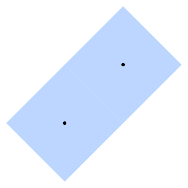
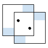
For example, suppose D=4 and there are repair centers at points (0, 0) and (5, 0). The point (0, 0) is non-distinguishable because Info(0, 0)={(0, 0)}=Info(5, 0). This means that point (5, 0) is also non-distinguishable. On the other hand, Info(3.5, 0.1)={(-3.5, -0.1), (1.5, -0.1)} is not equal to the information from any other point, which means that point (3.5, 0.1) is distinguishable. The following picture illustrates the regions of distinguishable points (in red) and non-distinguishable points (in blue):

Principia is deployed to a point that is chosen uniformly at random from the set of all points that are within D meters (using L1 distance) of at least one repair center — that is, the set of all points (x, y) such that Info(x, y) is non-empty. The probability of that choice belonging to a given continuous set of points S is proportional to the number of square meters of S's area. In the example above, each red square has an area of 4.5 square meters, while each blue section has an area of 23 square meters. Therefore, the probability of Principia being deployed within each red square is 4.5/(3×4.5 + 2×23) and the probability of it being deployed within each blue section is 23/(3×4.5 + 2×23). Since the border between adjacent differently-colored sections has area equal to 0, the probability of Principia being deployed exactly on the border is exactly 0.
Given the locations of all repair centers, what is the probability that the point to which Principia is deployed is distinguishable?
Input
The first line of the input gives the number of test cases, T. T test cases follow. Each test case starts with a line containing two integers N and D representing (respectively) the number of repair centers and the maximum L1 distance from which Principia can retrieve information from a repair center, as described above. Then, N lines follow. The i-th of these contains two integers Xi and Yi representing the coordinates of the i-th repair center. The unit of measurement for all coordinates and D is meters.
Output
For each test case, output one line containing Case #x: y z, where x is
the test case number (starting from 1) and y and z are non-negative
integers. The fraction y/z must represent
the probability of Principia being at a distinguishable location,
if one is chosen uniformly at random from all locations that are
within D meters of at least one repair center (using L1 distance).
If there are multiple acceptable values for y and z, choose
the one such that z is minimized.
Limits
Memory limit: 1GB.
1 ≤ T ≤ 100.
1 ≤ D ≤ 107.
-109 ≤ Xi ≤ 109, for all i.
-109 ≤ Yi ≤ 109, for all i.
(Xi, Yi) ≠ (Xj, Yj) for all i ≠ j.
(No two repair centers share the same location.)
Test Set 1 (Visible Verdict)
Time limit: 20 seconds.
N = 2.
Test Set 2 (Visible Verdict)
Time limit: 60 seconds.
2 ≤ N ≤ 10.
Test Set 3 (Visible Verdict)
Time limit: 120 seconds.
For 6 cases, N = 1687.
For T-6 cases, 2 ≤ N ≤ 100.
Sample
4
2 4
0 0
5 0
2 1
0 0
5 0
2 4
0 0
4 4
2 4
0 0
5 1
Case #1: 27 119
Case #2: 0 1
Case #3: 0 1
Case #4: 1 5
The above cases meet the limits for Test Set 1. Another sample case that does not meet those limits appears at the end of this section.
Sample Case #1 is described and depicted in the statement.
The points in the middle red region are all distinguishable points because they are the only points that retrieve information from both repair centers, and each point in that region retrieves a distinct set of information.
The points in the left and right red region each receive information from only one repair center, but that information is always unique, so these are all distinguishable points. For example, if Principia knows it is 3 meters east of a repair center, it can be sure it is not 3 meters east of the repair center at (0, 0), because then it would have retrieved information from both repair centers. So it must be 3 meters east of the repair center at (5, 0).
The points in the blue regions are all non-distinguishable points. Choose any point in one of those regions, and consider the information that Principia would get from that point. It contains only the one repair center in range. But, there is a corresponding point in the other blue region from which Principia would get exactly the same information.
As explained above, the probability of Principia being deployed to one of the red sections is 4.5/59.5, so the total probability of it being deployed to any of them is 3×4.5/59.5 = 27/119.
The following picture illustrates Sample Case #2. There is no way to retrieve information from
more than one repair center, so every point close enough to one of them is non-distinguishable;
the same information is retrieved from an equivalent point near the other one.
Remember that z (the denominator) must be minimal, so 0 1 is
the only acceptable answer.

The following picture illustrates Sample Case #3. Notice that the border between the two blue squares consists of distinguishable points. However, since its area is 0, the probability of Principia being deployed there is 0. All other points where Principia can be deployed are non-distinguishable.
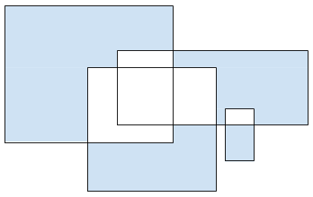
The following picture illustrates Sample Case #4.
The following picture illustrates the additional case.
The following additional case could not appear in Test Set 1, but could appear in any of the other test sets.
1
3 4
0 0
1 1
2 3
The correct output is Case #1: 101 109.
Analysis — A. Naming Compromise
Test Set 1
In Test Set 1, the limits are small enough that we might be tempted to just try lots of possible outputs and keep the best one. However, since there is no a priori limit on the output length, and we can use any of the English alphabet letters in the output, we need to think a little bit first. In addition, we have to actually implement the calculation of edit distance, which we can learn about via various online resources, including that Wikipedia link.
The distance between two strings of length up to 6 is at most 6, since we could just replace every character in the longer string (or an arbitrary one, if they are of the same length) to match the other string, and delete any excess. Moreover, the distance between two strings is never less than the absolute difference in length between them, because we would need to add at least that many characters to the shorter string (if one is indeed shorter) just to make it as long as the other string. It follows that the output should never be longer than 12 characters.
In addition, if the output N contains a letter
that is not present in either of the input strings, exchanging that letter in N for a letter
contained in one of the inputs cannot increase either distance, which can be proven by induction
by inspecting the recursive definition of edit distance. Therefore, we can limit our search
to strings of length up to 12 over the alphabet {X, Y, Z}.
There are less than a million candidates, and calculating the edit distance for such short
strings is really efficient, so this is fast enough to solve Test Set 1.
It is possible to prove tighter limits on the output, and this can drastically reduce the
number of candidates and make the solution even faster. We leave the details to the reader, but
consider whether we ever really need an answer longer than 6 letters. If we have
ABCDFG and ACDEFG, for example, then instead of compromising on the
seven-letter ABCDEFG by adding E to the first name and B
to the second name, we could just as easily delete B from the first name and
E from the second name, compromising on the shorter ACDFG instead.
Test Set 2
For Test Set 2 we need to use some additional insights. The most important one is noticing that edit distance is actually a distance, and has typical properties of distances like being reflexive and satisfying the triangle inequality. Let e(s, t) denote the edit distance between two strings s and t. For an output N, we want e(C, N) + e(J, N) = e(C, N) + e(N, J) to be minimal. By the triangle inequality, e(C, J) is a lower bound on this quantity, and an achievable one. For example, we can set N equal to C since e(C, C) = 0.
By the reasoning above, we need to find an N such that e(C, N) + e(N, J) = e(C, J) and |e(C, N) - e(N, J)| is as small as possible. Luckily, the definition of edit distance hints at a way of doing that. If the edit distance between C and J is d, it means that there is a path of d valid operations on C that results in it turning into J. Formally, there are d - 1 intermediate strings S1, S2, ..., Sd - 1 such that e(C, Si) = i and e(Si, J) = d - i. Therefore, it suffices to pick Sd / 2. If d is odd, both rounding up and down work, since for both possibilities, |e(C, N) - e(N, J)| = 1.
To find S1, S2, ..., Sd - 1, we can use a common technique to reconstruct the path that achieves an optimal result as found via dynamic programming (DP).
For example, let Ca be the prefix of length a of C and Jb be the prefix of length b of J. The usual algorithm to compute edit distance is based on a recursive definition of a function f(a, b) that returns e(Ca, Jb) (see the link from the previous section for details). Similarly, we can define g(a, b, k) as a fuction that returns e(Ca, Jb) and also a string S such that e(Ca, S) = k and e(Jb, S) = e(Ca, Jb) - k. The new function g can be defined with a similar recursion as f, and then memoized for efficiency. The details are left as an exercise for the reader.
Analysis — B. Thermometers
Test Set 1
First of all, notice that Xi splits the circle into a sequence of segments, so that throughout each segment, the temperature of all the points is the same. Let's say that the i-th segment is the segment which starts at Xi and goes clockwise. We will use di as the length of the i-th segment. Also note that per the problem statement, there are no adjacent segments with the same temperature, so we can safely ignore the actual temperatures Ti.
We can make the following observations:
- We never need more than two thermometers on each segment, as a thermometer put in between two others on the same segment will not cover any points which are not already covered by the original two.
- In an optimal answer, we should never have two adjacent segments with 2 thermometers each. If we have two adjacent segments with 2 thermometers in each, we can simply "push" the middle 2 thermometers outwards until at least one of them runs into the other thermometer in their segment, which reduces the total number of thermometers by at least one.
- The adjacent thermometers on different adjacent segments need to be equidistant from the common point of those segments. Otherwise, the temperature of some points between these thermometers will be incorrect.
- The thermometers in an optimal answer can always be put in integer or half-integer positions. If we have an answer in which that is not the case, we can "push" the thermometers until they reach integer or half-integer positions.
Given these observations, and the low limits in Test Set 1, we can iterate through all possible configurations and choose the one that gives the best answer.
Test Set 2
Note that if we know the position of a thermometer on segment A that is closest to an adjacent segment B, we can calculate the anticipated position of a thermometer on B. To do so, we need to "mirror" the known position over the common point of the segments. If the mirrored position doesn't belong to the segment B, then it is not possible for segment A to have the closest thermometer at this position.
First, let's assume that the answer is greater than N. We can apply the following greedy strategy to find the optimal answer (we will show below that it actually works).
Let's start with some segment A and assume that this is the only segment. We can put a thermometer at any point of A (except the endpoints, per the problem statement) and it will cover the whole segment. So the interval of valid positions on A is the whole segment. Now, let's consider an adjacent segment B and see how we can put the thermometers on both segments, so that only two thermometers are used. We can mirror the interval of valid positions in A over the common point of these segments. The interval of valid positions in B is the intersection of the mirrored segment and B. We will refer to this operation as propagation.
We can continue propagating this interval through as many segments as possible and stop if the propagated interval would be empty. If we propagate the last interval back to A through all the intermediate segments, this will give us valid positions for the thermometers to cover all these segments with one thermometer per segment.
As we cannot propagate the current interval anymore, we can define a new interval of valid positions on the current segment, taking into account the old one, effectively putting two thermometers on this segment, and repeat the process again. Once we reach segment A, we should verify that the last interval begins before the first interval ends, so that we could put two thermometers on segment A.
The answer will be N (as we have to put at least one thermometer on each segment) plus the number of times we had to start with the new interval, effectively putting two thermometers on the corresponding segment. We can try all segments as the starting one and choose the best answer. Again, the proof that this always works is given below.
Now let's see how to handle the case of the answer being equal to N, when we put exactly one thermometer on each segment. If we assume that zi is the position of a thermometer on segment i, measured from the segment's beginning (point Xi), then, we can calculate the other positions as follows:
z2 = d1 - z1
z3 = d2 - z2 = d2 - d1 - z1
...
zN = dN-1 - zN-1 = dN-1 - dN-2 + dN-3 - ... +/- z1
z1 = dN - zN = dN - dN-1 + dN-2 - dN-3 + ... +/- z1
These equations give us a quick test for whether the answer could be N.
In case N is even:
z1 = dN - dN-1 + dN-2 - dN-3 + ... - d1 + z1, or, subtracting z1 from both sides:
0 = dN - dN-1 + dN-2 - dN-3 + ... - d1
As long as the above holds, any z1 will satisfy the equation. The caveat here is that some of the zis may not be inside of the corresponding segments. So we need to verify that we can do the same propagation as we did earlier, and reach the first segment without adding the second thermometer on any segment. If we can do so, then the answer is N.
In case N is odd:
z1 = dN - dN-1 + dN-2 - dN-3 + ... + d1 - z1, or, adding z1 to both sides:
2z1 = dN - dN-1 + dN-2 - dN-3 + ... + d1
In this case, there is exactly one value for z1. As in the previous case, we need to verify that this value produces a valid set of positions, and we can do this by propagating z1 through all the segments. If we can do so, then the answer is N.
Propagating an interval through all segments is O(N), and we do this at most once to check N as an answer, and do this N times if the answer is not N. This gives us O(N2) running time.
Proof of greedy solution
Here is an image which roughly describes the steps in the proof below:

We will concentrate on the case when the answer is greater than N, since for the case of N the solution is constructive.
Let's define a few additional terms.
A chain is a sequence of adjacent segments, where there is some placement of thermometers such that each segment can be covered by one thermometer, except for the first and the last ones, each of which requires two thermometers. Note that it is possible that a chain covers the whole circle, starting in some segment, wrapping around the whole circle, and ending at the same segment.
A maximum chain is a chain that cannot be extended clockwise by adding the next segment because it is not possible to place the thermometers (as per the definition of a chain) to cover such a chain.
Two chains are consecutive if the last segment of one chain is the first segment of the other chain. Note that on the common segment, we will have to use two thermometers.
A valid sequence of chains is a sequence of consecutive chains containing all the given segments.
Note that any valid positioning of the thermometers is a valid sequence of chains, and the number of thermometers there is N plus the number of chains. The optimal answer is achieved in the positioning requiring the smallest number of chains.
Lemma 1. If we have a valid sequence of chains and the first chain is not a maximum chain, we can take some segments from the next chain(s) and attach them to this one until it becomes maximum, while keeping the sequence valid and not increasing the total number of chains.
Proof
Let's add a few more terms to our vocabulary.
The position of a thermometer on the i-th segment is the distance between the thermometer and Xi.
A chain flexibility interval is a set of valid thermometer positions on a segment of a chain, which can be correctly propagated through the whole chain. Note that it is always a subsegment (maybe of length 0) of a segment.
The first and last flexibility interval of a chain are the instances of the chain flexibility interval on the first and last segment of the chain accordingly.
We can now redefine a valid sequence of chains as a sequence of consecutive chains, containing all the segments, such that on every segment connecting two chains, if (xlast, ylast) and (xfirst, yfirst) are the last and first flexibility intervals of these chains, then xlast ≤ yfirst.
Now let's consider the first and second chains in some configuration:
- a, b and c are the lengths of the first, second and the third segments (if any) of the second chain. Note that a is also the last segment of the first chain.
- (x1, y1) - last flexibility interval of the first chain (on segment a).
- (x2, y2) - first flexibility interval of the second chain (also on segment a).
For clarity:
- x1 ≤ y2 by the definition of a valid sequence of chains.
- (a - y2, a - x2) - second flexibility interval of the second chain (on segment b).
Let's connect segment b to the first chain. Then:
- The last flexibility interval of the first chain will be mirrored to segment b and becomes (a - y1, min(b, a - x1)).
- The second flexibility interval of the second chain will become the first one, and in the worst case will be (a - y2, a - x2) (in other cases it will grow and will contain this interval fully).
First, let's consider the case where the initial flexibility intervals of the chains are intersecting (x2 ≤ y2). In this case the new configuration is valid, as a - y1 ≤ a - x2, so we can go on to try the next segment if possible.
Otherwise, if the original flexibility intervals were not intersecting (x2 > y1), then the new configuration is not valid. Again, the new flexibility intervals will be (a - y2, a - x2) and (a - y1, min(b, a - x1)), they will not intersect, and the first flexibility interval of the second chain will come before the last flexibility interval of the first chain (this is why the configuration is invalid).
However, we can notice that because (a - y2, a - x2) belongs to the second chain, it could be successfully propagated to the next segment (c) by definition. But, because (a - y1, min(b, a - x1)) is even closer to the segment border, we must be able to propagate it as well. This means that we can also attach the next segment to the first chain:
- The first flexibility interval of the second chain becomes (b - (a - x2), b - (a - y2))
- The last flexibility interval of the first chain will be (b - min(b, a - x1), min(c, b - (a - y1)))
Now the configuration is valid, because b - min(b, a - x1) ≤ b - (a - y2), and x1 ≤ y2 by definition.
What if we don't have a second segment to attach? Then we won't be able to attach the first one either, since the flexibility intervals were not intersecting, and the flexibility interval of a single segment is the whole segment.
Lemma 2. An optimal answer can always be achieved with a sequence of maximum chains and one potentially non-maximum chain.
Proof
Let's consider the first chain of an optimal answer. Let's attach segments from the next chain while we can (we are allowed to do so by Lemma 1). Repeat with the next chain, and so on. When we reach the last chain, leave it alone. Now all the chains except for the last one are maximum, and the last one can be either maximum or not.
The solution described above is building all possible sequences mentioned in Lemma 2, and by that lemma, some of them will be optimal.
Note that our proof has not dealt with small chains properly—that is, chains of length 1, 2 and 3 may not work properly in the proof above, but they are easy to deal with independently as special cases.
Analysis — C. Pen Testing
How to approach this problem?
At first sight, it might seem impossible to achieve the number of correct guesses required in this problem. If we just pick two pens at random without writing anything, the probability of success will be 46.666...%. And whenever we write anything, the amount of remaining ink only decreases, seemingly just making the goal harder to achieve. And yet we are asked to succeed in 63.6% of test cases in Test Set 3. How can we start moving in that direction?
Broadly speaking, there are three different avenues. The first avenue is solving this problem in one's head or on paper, in the same way most algorithmic problems are solved: by trying to come up with smaller sub-problems that can be solved, then trying to generalize the solutions to those sub-problems to the entire problem.
The second avenue is more experimental: given that the local testing tool covers the entire problem (i.e., there is no hidden input to it), we can start trying our ideas using the local testing tool. This way we can quickly identify the more promising ones, and also fine-tune them to achieve optimal performance. Note that one could also edit the local testing tool to make it more convenient for experimentation; for example, one could modify the interaction format so that only one test case is judged at a time.
The third avenue starts with implementing a dynamic programming solution that can be viewed as the exhaustive search with memoization: in each test case, our state is entirely determined by how much ink have we spent in each pen, and by which pens are known to have no ink left. Our transitions correspond to the basic operation available: trying to spend one unit of ink from a pen. Moreover, we can collapse the states that differ only by a permutation of pens into one, since they will have the same probability of success in an optimal strategy. Finally, we need to be able to compute the probability of success whenever we decide to stop writing and pick two pens; we can do this by considering all permutations, or by using some combinatorics (which is a bit faster). This approach is hopelessly slow for N=15. However, we can run it for smaller values of N and then use it as inspiration: we can print out sequences of interactions that happen for various input permutations, and then generalize what happens into an algorithm that will work for higher values of N.
Test Set 1
How can we find a small sub-problem in which writing actually helps improve the probability of success? Suppose we have only three pens, with 1, 9 and 10 units of ink remaining. If we just pick two pens at random, we will have two pens with at least 15 units of ink between them only with probability 1/3: 9+10≥15, but 1+9<15 and 1+10<15. However, if we first write 2 units of ink with each pen, we will know which pen had 1 unit of ink since we will fail to write 2 units with it, and will therefore know that the other two pens have 7 and 8 units of ink remaining, so we can pick them and succeed with probability 1!
How can we generalize this approach to the original problem? We can pick a number K and write K units of ink with each pen. Then, we will know the identities of pens 0, 1, ..., K-1 so that we can avoid taking them to the South Pole. However, the other pens will have 0, 1, ..., N-K units of ink remaining, which seems to be strictly worse than the initial state. But we can include a small optimization: we can stop writing as soon as we find all pens from the set 0, 1, ..., K-1. For example, if the two last pens both have at least K units initially, we will stop before we reach them, so by the time we identify all pens from the set 0, 1, ..., K-1 and stop writing, we will not have touched those two pens at all. Therefore we will know that they both have some amount of ink from the set K, K+1, ..., N, and picking them gives us a much higher probability of success. Of course, this will not always be the case, and sometimes we will have only one or zero untouched pens. In this case we should pick the untouched pen if we have it, and add a random pen from those that have written K units successfully.
By running this strategy against the local testing tool with various values of K, we can learn that it succeeds in about 56.5% of all cases when K=3, and is good enough to pass Test Set 1. We will call this strategy fixed-K.
There are certainly many other approaches that pass Test Set 1 — for example, less accurate implementations of the solutions for Test Set 2 and Test Set 3 mentioned below.
Test Set 2
How do we make further improvements? Our current approach suffers from two inefficiencies. The first inefficiency has to do with the fact that we keep writing K units of ink with each pen even if we have already found the pen which had K-1 units of ink initially. Since we are now searching for 0, 1, ..., K-2, it suffices to write only K-1 units of ink with each subsequent pen at this point. More generally, if X is the most full pen from the set 0, 1, ..., K-1 that we have not yet identified, we only need to write X+1 units of ink with the next pen. Having identified all pens from the set 0, 1, ..., K-1, we stop writing and take the two pens not from this set that have written the least units to the South Pole. We will call this improvement careful writing.
It turns out that careful writing with K=4 increases our chances substantially to 61.9%, enough to pass Test Set 2!
The second inefficiency is that out of the pens that are determined to have at least K units, we take two to the South Pole, but the rest are useless. For example, we never end up taking any pen except the last K+2 pens to the South Pole! Therefore we could start by writing with the first N-K-2 pens until they are used up and have exactly the same success rate. We can improve the success rate if we use the information that we get from those pens to make potentially better decisions!
More specifically, we can do the following: initially, write with the first pen until it is used up (and therefore we know how much ink was in it). Then, write with the second pen until it is used up, and so on. In this manner, we will always know exactly which pens are remaining. At some point we should decide to stop gathering information and switch to the fixed-K strategy. The information we gathered can be used to pick the optimal value of K, which is potentially different in different branches.
This gives rise to a dynamic programming approach with 2N states: a state is defined by the set of pens remaining after we have used up some pens. For each state we consider either writing with the next pen until it is used up, or trying the fixed-K strategy with each value of K. Note that we only need to run the dynamic programming once before the interaction starts, and then we can use its results to solve all test cases.
We will call this improvement to the fixed-K strategy pen exploration. It turns out that pen exploration allows us to succeed in about 62.7% of all cases, which is also enough to pass Test Set 2. We expect that there are many additional ways to pass it.
Test Set 3
What about Test Set 3? You might have guessed it: we can actually combine careful writing and pen exploration! This yields a solution that succeeds in about 63.7% of all cases, which is close to the boundary of Test Set 3, so while it might not pass from the first attempt because of bad luck, it will definitely pass after a few attempts.
This is not the only way to solve Test Set 3, though. If we take a closer look at the careful writing solution, we can notice that we can achieve exactly the same outcome using a bottom-up approach instead of a left-to-right approach. More specifically, we start by writing one unit of ink using each pen in the order from left to right, until we find a pen that cannot write; we can conclude that it is the pen that started with 0 units of ink. Then, we can go from left to right again and make sure that each subsequent pen has written two units of ink (which will entail writing one more unit of ink from pens that have already written one, or writing two units of ink for pens that were untouched in the last round), until we find the pen that had 1 unit of ink in the beginning. We continue in the same manner until we have found pens 0, 1, ..., K-1, just as before. The amount written with each pen at this point will be exactly the same as the amount written with each pen in the original careful writing approach.
However, this formulation allows us to improve this approach: we no longer need to pick K in advance! We can instead make a decision after finding each pen X: either we continue by searching for the pen X+1 in the above manner, or we stop and return the two pens that have written the least so far. We will call this improvement early stopping. In order to make the decision of whether to continue or to return, we can either implement some heuristics, or actually compute the probability of success using a dynamic programming approach where the state is the amount written by each pen at the time we have found pens 0, 1, ..., X. This dynamic programming has just 32301 states for N=15, so it can be computed quickly.
Careful writing with early stopping works in about 64.2% of all cases if one makes the optimal decisions computed by the aforementioned dynamic programming, allowing one to pass Test Set 3 with a more comfortable margin. Once again, we expect that there are many additional approaches available for Test Set 3.
Ultimate solution
All three improvements — careful writing, pen exploration and early
stopping — can be combined in one solution. It is a dynamic programming solution in
which the state is once again the amount written with each pen, and we consider three options for
every state:
1. Write with the leftmost remaining (=not known to be used up) pen until it is used up.
2. Write with all pens from left to right to find the smallest remaining pen.
3. Return the two rightmost pens that have not been used up yet.
Note that computing the probability of success for the third option is easy in this solution, as each of the remaining pens can be at any of the available positions. This means that any pair of remaining pens is equally likely to appear as the two pens we are taking to the South Pole. This means, in turn, that if the pens we are taking to the South Pole have written X and Y units, then the probability of success is simply the number of pairs of remaining pens with initial amounts A and B such that A+B>=N+X+Y, divided by the total number of pairs of remaining pens.
This dynamic programming has 1343425 states for N=15; therefore, it can run in time even in PyPy if implemented carefully. Its probability of success is around 64.4%, which is more than enough for Test Set 3.
Moreover, we have compared the probability of success for this approach with the optimal one (computed by the aforementioned exhaustive search with memoization, after a lot of waiting), and it turns out that for all N≤15 this solution is in fact optimal. Therefore, we suspect that it is optimal for higher values of N as well. We do not have a proof of this fact, but we would be very interested to hear it if you have one! Of course, neither this solution nor its proof are necessary to pass all test sets in this problem.
Constraints and judge
Finally, let us share some considerations that went into preparing the constraints and the judge for this problem. Given its random nature, the fraction of successfully solved test cases will vary for every solution. More specifically, thanks to the Central Limit Theorem we know that for a solution with probability of success P that is run on T test cases, the fraction of successfully solved test cases will be approximately normally distributed with mean P and standard deviation sqrt(P×(1-P)/T). In Test Sets 1 and 2 the standard deviation is therefore around 0.35%, and in Test Set 3 it is around 0.15%.
Considering the probabilities that a sample from a normal distribution deviates from its mean by a certain multiple of its standard deviation, we can see that for practical purposes we can expect to never land more than, say, five standard deviations away from the mean. This creates a window of about ±1.75% in Test sets 1 and 2, and a window of about ±0.75% in Test Set 3 such that whenever a solution is outside this window, it will always pass or always fail, but within this window the outcome depends on luck to some degree.
This luck window is inevitable and its size almost does not depend on the required success rate, only on the number T of test cases. Therefore it is impossible to completely avoid the situation when the success rate of a solution falls into the luck window, and therefore one might need to submit the same solution multiple times to get it accepted, with the number of required attempts depending on luck. Increasing the number T reduces the luck window, but increasing it too much requires the solutions to be extremely efficient and can rule out some approaches. Therefore, we decided that the best tradeoff lies around T=20000 for Test Sets 1 and 2, allowing less efficient approaches to still pass there. For Test Set 3, we felt the best tradeoff lies around T=100000 to better separate the solutions that are optimal or close to optimal from the rest and to reduce the luck window, while still not pushing the time limit to impractical amounts.
We have picked the required success rates in the following manner:
- For Test Set 1, we picked it such that the fixed-K strategy is outside the luck window and
always passes.
- For Test Set 2, we picked it such that both careful writing and pen exploration are outside
the luck window and always pass.
- For Test Set 3, we picked it such that the ultimate solution with all three improvements
is outside the luck window and always passes, but solutions with careful writing and one of
early stopping or pen exploration are within the luck window and therefore might require
multiple submissions, but not too many. Lowering the threshold further in this test set
would bring pen exploration without careful writing within the luck window. More generally,
there is a continuum of solutions here if one uses inexact heuristics instead of exact
dynamic programming to make the early stopping decision, and some of those solutions
would inevitably land in the luck window.
Another peculiar property of this problem is that the judge is not deterministic, whereas typically in interactive problems, the randomness in each test set is fixed in advance, and submitting the same deterministic code always leads to the same outcome. This is necessary to avoid approaches in which one first uses a few submissions to learn some information about the test sets, for example by making the solution fail with Wrong Answer or Runtime Error or Time Limit or Memory Limit, to pass two bits of infomation back. This information can then be used to achieve a higher probability of success.
In order to see how this small amount of information can help significantly, consider a solution that has a probability of success that is five standard deviations smaller than the required one. Using the simple "submit the same code again" approach, one would need more than 3 million attempts on average to get it accepted, which is clearly not practical. However, we can do the following instead: we can submit a solution that just writes with all pens until they are used up, therefore gaining full knowledge of the test set. Then, it runs the suboptimal solution several million times with different random seeds, which by the above argument will find a random seed where the suboptimal solution in fact achieves the required success rate. Now the solution just needs to communicate back 20-30 bits comprising this random seed, which even at the two bits per submission rate requires just 10-15 submissions, which can be made within the space of a round. Finally, one could just submit the suboptimal solution with this random seed hardcoded, and pass.
We hope that this provides some insight into why this problem is designed the way it is, and we are sorry that some potential remained for contestants to be negatively impacted by the luck window or by the judge's non-determinism.
Analysis — D. Recalculating
A quarter pi helps the math go down
As can be seen in the pictures in the statement, lines dividing distinguishable and non-distinguishable areas are always 45 degree diagonals. The reason is that the distinguishability can only change when the retrievability of some repair center changes, and those only change when crossing diagonals because of the sum in the L1 distance definition. Since horizontals and verticals are much easier to deal with than diagonals, we can rotate the whole problem by π/4 = 45 degrees. If we do that directly (for example, by multiplying all points by the corresponding rotation matrix) we will find ourselves dealing with points at non-integer coordinates, which has problems in itself. Notice that rotating is equivalent to projecting into new axes of coordinates. In this case, the directions of those new axes are the rows of the rotation matrix, or (2-2, 2-2) and (2-2, -2-2). The vectors (1, 1) and (1, -1) have the same directions but do not have length 1. We can still project onto them and end up with a rotated and re-scaled version of the input. Luckily, neither rotation nor re-scaling affects the ultimate result. So, a convenient transformation is to map each point (x, y) in the input to (x+y, x-y). Notice that in this rotated and scaled world, L1 distance changes to L∞ distance, which is just a fancy way of saying that those diagonals turn into horizontals and verticals that are exactly D meters away from the point in question. Although we will not explicitly mention it, this transformation is applied as the first step of all solutions presented here.
Test Set 1
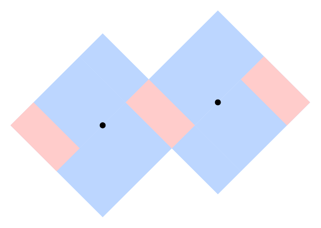
We can write a solution for Test Set 1 by examining a few cases and finding a formula for each one. The set of points from which a repair center can be seen is an axis-aligned square of side 2D with the repair center at its center. Let us call that the r-square of the point.
There are 3 possible situations:
- I: The r-squares do not intersect.
- II: The r-squares intersect and the repair centers are outside each other's r-squares.
- III: The repair centers are inside each other's r-squares.
Situation I is the easiest to handle, because the answer is always 0, as Sample Case #2 illustrates.
Situation II is illustrated by Sample Case #1. As suggested in the statement, we can find the red area as 3 times the area of the intersection of both r-squares (notice that the intersection is not necessarily a square) and the blue area as the sum of both r-squares, 2×(2D)2, minus the area of the intersection.
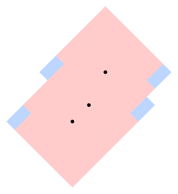
In Situation III, the total area in which Principia could be deployed can be calculated in the same way as before. The distinguishable area, however, is slightly different. It can be simpler to calculate the non-distinguishable area (highlighted below), which consists of four copies of the same region, and then complement the result.
Test Set 2
Recall that Info(p) is the set of relative locations of repair centers that can be retrieved from a point p. Notice that when two points p and p' are very close, Info(p) and Info(p') will look similar. If the repair centers that can be retrieved from both are the same (which is true most of the time for points that are close to each other), then Info(p') is equal to Info(p) shifted by the shift between p and p'. However, if at least one repair center is retrieved from one of these points and not from the other, that is not true. In particular, Info(p) and Info(p') could be sets of different numbers of points.
First we deal with the changes in which repair centers can be retrieved by splitting the interesting area into parts. Within each part, the set of repair centers that can be retrieved is constant. Consider all the horizontal lines y=X+D and y=X-D for each x-coordinate X of a point in the input, and all vertical lines x=Y+D and x=Y-D for each y-coordinate Y of a point in the input. The points that are not surrounded by 4 of these lines (for example, the points above the highest horizontal line) are too far from all of the repair centers to be able to retrieve any of them, so we can disregard them for the rest of the analysis. These up to 4N lines divide the remaining points into up to 4N2 - 4N - 1 rectangular regions. Since all sides of all r-squares fully overlap with these lines, the set of repair centers that are retrievable from any point strictly within one of those regions is the same. The set of repair centers that can be retrieved from points on the lines might be different from those retrieved from any of its adjacent regions. However, since the area of each line is 0, the probability of Principia being deployed there is 0, so we simply ignore them and work with points strictly within regions. For each region R, we calculate the total area A(R) of distinguishable points in the region and the total area B(R) of points where Principia can be deployed. The answer is then the sum of A(R) over all regions divided by the sum of B(R) over all regions.
Fix a current region C. Going back to the first paragraph, Info(p) and Info(p') are shifts of each other for all p and p' from the same region. Calculating B(C) is easiest: it is either the area of C if Info(p) is non-empty for any point p in the region, and 0 otherwise. To calculate A(C), we can use an analysis generalizing our reasoning in Test Set 1. We need to find other regions R where Info(q) is a shift of Info(p) for a point q in R. In Test Set 1, this happened for the regions where one repair center can be seen, because the sets of a single point are always shifts of each other. We can check whether Info(p) and Info(q) are shifts of each other and find the appropriate shift if they are. First we check that they have the same number of points, and then we sort the points in an order that is invariant by shift (for example, sorting by x-coordinate and breaking ties by y-coordinate). In this way, we can fix the shift as the one between the first point of Info(p) and the first point of Info(q). Finally, we check that that shift works for all pairs of i-th points. If true, we can shift R by the found amount to obtain R', and the intersection between R' and C is a rectangle in which the points are non-distinguishable. If we do that over all regions R, the union of all those intersections is exactly the area of non-distinguishable points in C, and we can subtract it from the area of C to obtain B(C). There are many algorithms (with different levels of efficiency) to find the area of the union of rectangles aligned with the axes. Given the low limits of Test Set 2, it suffices to use a technique like the above, in which we extend the rectangle sides to lines and divide into regions, checking each region individually.
For each region C, the algorithm needs to find Info(p) for a point p in C, which takes time O(N), then iterate over all other O(N2) regions R and find Info(q) for a point there, check Info(q) against Info(p) for a shift, and possibly produce an intersection. That takes O(N) time per R, or O(N3) overall for the fixed C. Then, we need to take the union of up to O(N2) rectangles, which, with the simple algorithm above, can take between O(N4) and O(N6) time, depending on implementation details. This means the overall time, summing over all possible C, can be up to O(N8). Most implementations should be OK in most languages though. As we will see, there are many optimizations needed for Test Set 3, and even just doing the simplest of them would be enough to pass Test Set 2. Alternatively, there is a known algorithm to find the area of the union of K rectangles in O(K log K) time, and multiple references to it can be found online. Using it off the shelf would yield an overall time complexity of O(N4 log N), which is small enough to handle much larger limits than Test Set 2's.
Test Set 3
To solve Test Set 3, we have a lot of optimization to do. The first step is to avoid calculating Info for each region more than once. That alone does not change the ultimate time complexity of the algorithm from the previous section, but it is a necessary step for all optimizations that follow.
We divide the work into two phases. In the first phase, we group all regions that have equivalent Info sets. For each region C, we calculate S := Info(p) for an arbitrary point p in C as before, discard it if S is empty. Otherwise, we sort S, and then shift both C and the sorted result by the first point such that the shifted S' has the origin as its first point. In this way, S' is a normalized pattern for C, and two regions with Info sets that are shifts of each other end up with the same S. After doing this, we can accumulate all shifted regions for each S that appears, and process them together.
Notice that we can sort the input points at the very beginning and then always process them in order such that every calculated S is already sorted, to avoid an extra log N factor in the time complexity. A rough implementation of this phase takes O(N3) time if we use a dictionary over a hash table to aggregate all regions for each set S. We optimize this further below.
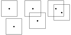
For the second phase, we have to process the set of shifted regions for each shifted S'. Since the regions are already shifted in a normalized way, we can process them all together. That is, instead of calculating A(C) for each individual C, we calculate A(S') := the sum of A(C) over all C in S'.
The picture below shows an example of the input we need to process for a fixed S'. There are multiple rectangular regions that have been shifted, so some may overlap now. We need the area of the part where no intersections happen (highlighted in the picture). If we do this by extending sides and processing each resulting region individually, we end up with an algorithm that takes between O(K2) and O(K3) time again, where K is the number of rectangles. However, the sum of the number of rectangles over all S' is O(N2), because each original region appears in at most one group. Therefore, the overall cost of the second phase implemented like this over all S' would be between O(N4) and O(N6).
We now have an algorithm with a first phase that takes O(N3) time and a second phase that takes between O(N4) and O(N6) time overall. We need to optimize further.
For the first phase, if we want to keep O(N2) regions and go significantly below O(N3), we need to make the processing of each region not require a full pass over the input points. Consider a fixed row of regions between the same two horizontal lines. Notice that each repair center can be retrieved from a contiguous set of those regions, and they become both retrievable and non-retrievable in sorted order of x-coordinate. Therefore, we can maintain the list of points that represent S in amortized constant time by simply pushing repair centers that become retrievable to the back of the list and popping repair centers that become non-retrievable from the front. This technique is sometimes called "chasing pointers".
Unfortunately, this is not enough, as we need to shift each S by a different amount, and shifting S requires time linear in the size of S. It is entirely possible for S to contain a significant percentage of points for a significant percentage of regions. We can do better by using a rolling hash of S. That would get us a hash of each S without any additional complexity. Unfortunately, we cannot shift the resulting hash. The last trick is, instead of hashing the actual points, hash the shift between each point and the last considered (adding a virtual initial point with any value). Those internal shifts are invariant to our overall shift of S, and since the first point of S' is always the origin, we can simply remove that one from the hash. The result is something that uniquely (up to hash collisions) represents the shifted S'. This change optimizes the first phase to run in O(N2) time.
To optimize the second phase — specifically the calculation of the values A(C) — we can use an algorithm similar to the one mentioned at the end of the previous section to calculate the union of the area of all rectangles. Consider a sweep line algorithm that processes the start and end of each rectangle in order of x-coordinate. We can maintain a data structure that knows, for each y-coordinate, how many rectangles overlap the sweep line at coordinate y. We need to be able to insert a new interval of y-coordinates each time a rectangle starts, remove one each time a rectangle ends, and query the total length of y-coordinate covered by exactly one rectangle. Multiplying that by the difference in x-coordinate between stops of the sweep line, we can calculate how much area to add to A(S') at each stop of the sweep line.
We can use a segment tree to efficiently represent that. At each node of the segment tree we need to record:
- (1) How many rectangles processed so far fully cover the interval represented by the node and do not fully cover its parent.
- (2) The total length covered by 1 or more rectangles within the interval represented by the node.
- (3) The total length covered by 2 or more rectangles within the interval represented by the node.
Since each insertion and removal requires going through at most O(log K) nodes, and the queries are resolved in constant time, using this sweep line algorithm with the described segment tree structure results in an algorithm that processes a set of K rectangles for the second phase in O(K log K) time. This results in O(N2 log N) time overall for the phase (and the algorithm), since, as we argued before, the sum of all K over all S' is O(N2).