Google Code Jam Archive — Round 3 2017 problems

Googlements: Analysis

Small dataset

In the Small dataset, the googlements can have a maximum length of 5. We will discuss googlements of that length; the procedure for shorter ones is the same.

Any string of length 5 that uses digits only in the range [0, 5] and is not 00000 is a googlement; there are 6⁵ - 1 = 7775 of these. One workable solution is to iterate through all of these possible googlements and simulate the decay process for each one until it reaches the sole possible looping end state of 10000. As we do this, for each googlement, we maintain a count of how many decay chains it appears in. When we are finished, we will know how many possible ancestors each googlement has, and so we will have the answer to every possible Small test case!

Later in this analysis, we will show why 10000 is the only googlement of length 5 that is its own descendant, and we will look into how long a decay chain can go on. Even if each chain were somehow as long as the number of googlements, though, with only 7775 googlements, this method would still easily run fast enough to solve the Small.

That approach is "top-down"; a "bottom-up" approach to this tree problem also works. For a given googlement, we can figure out what digits must have been in the googlement that created it (its "direct ancestor"). For example, if we are given 12000, we know that any direct ancestor must have one 1, two 2s, and two 0s to bring the total number of digits to five. Then we can create all such googlements (e.g., 12020) and recursively count their direct ancestors (e.g., 42412) in the same way. This process does not go on forever, because (as we noted above) there are at most 7775 googlements in the tree. The worst-case scenario is 10000, which is a descendant of every googlement.

After thinking through the bottom-up approach, only implementation details remain. The toughest part is generating direct ancestors with particular counts of particular digits. A permutation library can help, or we can write code to generate permutations in a way that avoids repeatedly considering duplicates. We can save some time across test cases by memoizing results for particular nodes of the tree, since the decay behavior of a given googlement is always exactly the same, and some of the same googlements could (and probably will) show up many times in different cases.

Large dataset

In the bottom-up Small approach outlined above, we spent a lot of time generating new direct ancestors to check. For ancestors such as 12020 that themselves had direct ancestors, this was necessary. However, it was a waste of time to construct and enumerate ancestors such as 42412, which have no ancestors of their own. More generally, a googlement of length L with a digit sum of more than L cannot have any ancestors, since it is impossible to fit more than L digits into a length of L.

It turns out that avoiding enumerating these ancestor-less ancestors saves enough time to turn that bottom-up Small solution into a Large solution. We can do that with some help from combinatorics and the multinomial theorem.

Let's think again about the direct ancestors of 12020. Each must have one 1, two 2s, and two 4s. How many ways are there to construct such a string? Starting with a blank set of 5 digits, there are (5 choose 2) = 10 ways to place the 2s, then (3 choose 2) = 3 ways to place the 4s into two of the three remaining slots, then (1 choose 1) = 1 ways to place the leftover 1. These terms multiply to give us a total of 30 ways, so 12020 has 30 direct ancestors. Since each has a digit sum of 13, which is greater than 5, none of them have their own ancestors. So we do not care what they are; we can just add 30 to our total.

At this point, we can either test this improvement on the worst-case googlement 100000000 before downloading the Large dataset, or we can reassure ourselves via more combinatorics. The googlements of length 9 with ancestors are the ones with a digit sum less than or equal to 9; we can use a balls-in-boxes argument to find that that number is (10 + 9 - 1)! / (10! * (9-1)!), which is 92377. This is a tiny fraction of the 999999999 possible googlements of length 9; we have avoided enumerating the other 999900000 or so! As long as our method for generating ancestors doesn't impose too much overhead, this is easily fast enough to solve 100 Large test cases in time, even if most or all of them explore most or all of the tree.

Appendix: Some justifications

Let's prove that there is only one looping state for a given googlement length, and that there are no other loops in the graph. We will start with some observations.

• When a googlement decays, the number of non-0 digits in the googlement equals the sum of the digits in the googlement it decays into.
• Because of this, any googlement that has a digit other than 0s or 1s will decay into a googlement with a smaller digit sum.
• Any googlement consisting only of 0s and 1s will decay into a googlement with the same digit sum. If the googlement is 1 followed by zero or more 0s, it will decay into itself. If the googlement has a single 1 at another position, it will decay into a 1 followed by 0s. Otherwise, it must have at least two 1s, so it will decay into a googlement with the same digit sum but with at least one digit other than 0 or 1.

We can draw some useful conclusions from the above observations:

• The only googlement of length L that can decay into itself is a 1 followed by L-1 0s. For any other googlement, decay would either reduce its digit sum or create a new googlement with a digit other than 0 or 1, which would itself decay into a googlement with a smaller digit sum.
• It can take at most two steps for a chain of googlements to lose at least one point of digit sum. This puts a bound on the height of the decay tree; it can be at most 2 times the maximum possible digit sum. (Moreover, it is even less than this; for example, a googlement of 999999999 will immediately decay into 000000009, losing a large amount of its digit sum.

Good News And Bad News: Analysis

The ordered pairs of friends form a directed graph in which each friend is a node and each news path is an edge. Notice that we can work on one connected component at a time, because each can be solved independently of the others. In the following, we assume a connected graph.

One additional observation is that if any edge of the undirected graph is a bridge — that is, an edge not present in any cycle — then the task is impossible. This is a consequence of the news balance on nodes extending to subsets of nodes: if we group nodes on each side of the bridge, the aggregate balance of each subset must be zero, and values in edges internal to the subset don't affect that balance. Since the bridge is the only external edge, this forces its value to be zero. Formally, the news balance property is preserved by vertex identification, and we can identify all vertices on each side of the bridge to reach a contradiction.

Note that since we can pass positive or negative news on each edge, we can forget about the directions of edges in our graph, and consider it as undirected. If the directed version had opposing edges (v, w) and (w, v), the undirected version can just have two edges between v and w. After solving the problem on the undirected graph, we simply adjust the sign of the value we assign to each edge according to its original direction.

Small dataset

The Small dataset can have up to 4 friends, so there can be as many as 12 edges. The bad news is that with up to 2 × 4² = 32 possible legal values for each of those edges, there can be 32¹² possible answers to check, which is far too large to handle with brute force. The good news is that there are only on the order of 2¹² graphs to consider; we can rule out the ones that have bridges (since those are impossible), and then run whatever method we come up with on all of the others to see if we get solutions.

What if we don't really need the full extent of the [-16, 16] range? We can try restricting our values to a smaller set and see whether we get solutions. As Sample Case #5 demonstrates, we might need negative values, so we can try a set like {-2, -1, 1, 2, 3}, for instance. It turns out that this set alone is enough to solve all possible Small cases that do not contain a bridge, so we can use brute force to find all possible assignments.

Large dataset

Judging by the Small solution, we may believe that all bridgeless graphs do have a solution, and that's indeed the case (as we will see in Solution 2, below).

Solution 1. Start by using depth-first search to build a spanning tree of the underlying undirected graph. Assign all non-tree edges a random nonzero value in [-K, K]. Now, the current balance of each node is some integer. In leaf-to-root order, we can go through all nodes using the single non-assigned edge remaining to make the balance zero. Notice that if we fix all F-1 non-root nodes, the root is automatically fixed, because the sum of the balance over all nodes always equals 0 (an edge with value v contributes v to one balance and -v to another). Notice that it is possible that a node's balance is 0 when we need to fix it, leaving us no non-zero choice for the corresponding tree edge. Additionally, if the balance on a node is too high, the value we need for the corresponding edge could be out of range. However, a value for K around F yields a small probability of both, which we can find through experimentation. And, if we happen to run into a problem, we can re-run the algorithm. As long as the probability of success is a not-too-small constant, running it enough times will eventually yield a valid assignment. Since we can implement this in linear time, and the bounds are small, we can afford thousands of runs per test case, or possibly more. So, even with weak experimental data on the probabilities, we can build enough confidence that this method works. Notice that we can avoid explicitly checking for bridges by assuming that failure after 1000 or so retries means the case is impossible.

Solution 2. Again, find a DFS spanning tree of the graph and number the nodes in discovery order. Remember that in a DFS over an undirected graph, every non-tree edge goes from a node to some ancestor in the tree. Direct all edges in root-to-leaf direction (we reverse or split edges after solving, as explained above). We assign edges not in the tree a value of 1, that is, they send positive news from nodes to descendants. On the other hand, we assign negative values to tree edges. We process the nodes in reverse discovery order: as in the previous randomized solution, each node has a single adjacent edge with no assigned value, so we assign it the only value that makes the node balanced.

Let us prove that the values assigned this way are all negative if there is no bridge or contain a zero if there is a bridge: assume a value of 0 for unassigned edges to check the current balance of a node x right before we attempt to balance it. Let A be the set of descendants of x, including x itself. There is exactly one tree edge going into A: the edge that we are trying to assign at this step. Let us call it e. All other edges going into A are non-tree, so they all have a value of 1. The current aggregate balance of A then equals the number of non-tree edges going into A. Since nodes are processed in leaf-to-root order, all nodes in A other than x are balanced, and A's balance equals x's balance. If the number is zero, then there are no edges other than e going into A, which makes e a bridge. If the number is greater than 0 (it is a number of edges, so it can't be negative), the current balance of x is greater than 0 and we can assign its opposite, a negative number, to e. This value is always within the legal [-F², F²] range, because its magnitude is equal to some number of edges in the graph, and the total number of edges in the graph cannot exceed F × (F - 1), which is less than F².

Solution 3. We keep the nodes balanced at all times. Start with 0 on all edges. For each undirected edge, if it has a 0 in the current valuation, find a cycle that contains it and then add -K to all edges of the cycle, where K is an integer different from the current values of all edges in the cycle. This choice of K guarantees that the procedure doesn't change a non-zero edge into zero, and it always changes at least one zero edge into a non-zero (the current edge), so it always finishes. Adding a value to edges in a cycle maintains the balance of each node. If we choose K with minimum possible absolute value, and cycles as short as possible, this won't exceed the range. The easy to prove maximum absolute value this can produce is F × P / 2, because K is always in the range [-F/2, F/2] as there can't be more than F forbidden values for it. There are also at most P steps. However, there are many results showing that graphs with many edges have lots of short cycles, so we believe it's impossible to construct a case in which the range is exceeded. Further, if we randomize the order to fix edges and retry many times, we can work around the worst cases that specifically try to overload a given edge, but possibly produce lots of small cycles that help fix the others cheaply. Notice that the idea of using the DFS tree to fix balances in the previous solutions is actually the same idea from this theoretically simpler solution, but using the fundamental cycles of the graph instead of potentially all of them.

Mountain Tour: Analysis

Small dataset

Since each hiking tour can be taken only once, each of the hiking tours arriving at a camp must be followed by a different departing tour. Since each camp has two arriving and two departing tours, there are exactly two ways to “pair” the hiking tours at a camp: the first arrival with the first departure (and the second arrival with the second departure), or the first arrival with the second departure (and the second arrival with the first departure). We can think of a candidate solution as specifying this boolean decision for each camp. The total duration is the sum of each hiking trip's duration and the amount of time waiting at each camp.

When evaluating a possible solution, you must check whether or not every hiking tour is present on the path beginning with your start hike. It is possible for a path through the graph to represent a cycle with fewer than 2C edges. For example, the left side of the figure farther down on the page shows a setup with three disjoint paths through the graph.

Because the time spent waiting at the base camp is calculated differently than the time spent waiting at all other camps, the base camp needs to be handled as a special case. You could simply run the algorithm four times, once for each “start” and “end” hike.

The entire space can be explored in O(2^C) time, which is sufficient for the Small dataset with C ≤ 15.

Another way to look at the small dataset is as a special case of the Travelling Salesman Problem (TSP). Consider the directed graph in which each hiking tour is a node and edges are the possible pairings between hiking tours, four for each camp, with edge weights corresponding to the amount of time you would have to wait at the camp in order to make that transfer. For example, if hiking tour A arrived at node 1 at time 02:00, and hiking tour B left node 1 at time 06:00, there would be an edge from A to B with weight 4. Running TSP on this graph, again with special handling for the base camp, can also yield a correct solution.

Large dataset

Let's look more closely at the two possible arrival-departure pairings for each camp. Suppose a camp has tours arriving at 13:00 and 21:00 and tours leaving at 22:00 and 07:00, such that there are no departures between the times that the two tours arrive. If the 13:00 arrival were paired with the 22:00 departure and the 21:00 arrival were paired with the 07:00 departure, the total wait time at the camp would be (22 – 13) + ((7 – 21) mod 24) = 19 hours. If we did the other pairing, the total wait time would be (22 – 21) + ((7 – 13) mod 24) = 19 hours. Both pairings result in the same total wait time at the camp. We will call these camps the “free” camps.

Now consider a camp having tours arriving at 11:00 and 23:00 and tours leaving at 17:00 and 08:00, such that after each tour arrives, there is a tour that leaves before the other tour arrives. If the 11:00 arrival were paired with the 17:00 departure and the 23:00 arrival were paired with the 08:00 departure, the total wait time at the camp would be (17 – 11) + ((8 – 23) mod 24) = 15 hours. If we did the other pairing, the total wait time would be ((17 – 23) mod 24) + ((8 – 11) mod 24) = 39 hours, 24 hours longer than the other pairing.

We mentioned that for the small solution, you must ensure that every hiking tour is present on the path starting from the base camp. What does the graph look like if there are hiking tours that are not present on that path? It is a set of disjoint cycles. Each camp has two paths crossing through it. If those paths are on different cycles, switching the pairing of that camp will in effect merge the two cycles together.

For example, consider the following figure with 5 camps. Camps 2 and 5 are free, and camps 3 and 4 are 24-hour switches. The initial graph has 3 disjoint cycles. As it turns out, to merge all of the cycles together, it is necessary to switch the pairing of camp 5 for free and either camp 3 or camp 4 for a 24-hour penalty. Note that the red path, the one starting and ending at the base camp, does not pass through camp 5 prior to switching the pairings, but switching the pairing of camp 5 is nonetheless required.

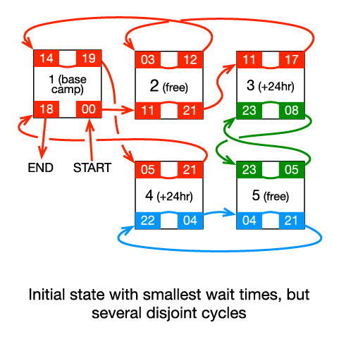
In this initial state, wait times are minimized, but there are several disjoint cycles.

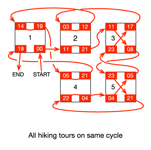
Now there is only one cycle.

Thus, to solve the problem efficiently, add each hiking tour to a Disjoint Sets data structure. Iterate through each camp. If the camp is free, union all four hiking tours connected to that camp into the same set (this is analogous to letting the free camps take either pairing); otherwise, union each arrival with only its respective departure. You will end up with one disjoint set per cycle in the graph. If there are Q > 1 disjoint sets, since all of the free camps have already been accounted for, you will need to switch the pairing of Q – 1 camps with 24-hour penalties. These Q – 1 camps are guaranteed to exist. The base camp still needs special handling; you can afford to run the algorithm once for each of the four possible start and end hikes. The total duration is the sum of all the hiking tour durations plus the lowest waiting time at each camp plus 24 hours for each of the Q – 1 penalties. This solution takes O(C α(C)) time, where α(C), the inverse Ackermann function, is the amortized time per operation on the Disjoint Sets data structure.

Slate Modern: Analysis

Small dataset

To formalize the reasoning about this problem and yield both an algorithm and a proof of its correctness we will resort to some graph theory. Consider an undirected graph G where the set of R × C + 1 nodes is the set of cells in the painting plus an additional special node we call root. We add an edge between each pair of adjacent cells with length D and for each cell that has a fixed brightness value v we add an edge from the root to the cell node with length v.

Let p(c) be the length of the shortest path on G from the root to the node that represents cell c.

Property 1. The p(c) is an upper bound on the value that can be assigned to c. Let
root, a₁, a₂, ..., a_k=c
be the path of k edges from the root to c of total length p(c). By construction of G, a₁ is a fixed cell. Let v be a₁'s value. Also by construction, the edge (root, a₁) has length v and all other edges (a_i, a_i+1) have length D. Thus, p(a_i) = v + (i - 1) × D. Clearly p(a₁) = v is an upper bound on its value v, and by induction, if p(a_i) is an upper bound on the values that can be assigned to a_i, p(a_i+1) = p(a_i) + D is an upper bound on the values that can be assigned to a_i+1 because it can't differ by more than D with the value assigned to a_i because the corresponding cells are adjacent (any edge from G not involving the root connects nodes representing adjacent cells).

Property 2. Let c be a fixed cell with value v. If p(c) ≠ v, then the case is impossible. Since there is an edge (root, c) with length v, p(c) ≤ v. And, if p(c) < v, the case is impossible by Property 1.

Property 3. If p(c) is exactly the value assigned to c for all fixed cells c, then the case is possible and assigning p(c) to each non-fixed cell c is a valid assignment of maximum sum. By the precondition we know that p assigns all fixed-cells their original value, so we only need to check if neighboring cells are assigned values that differ by no more than D. Let c and d be two neighboring cells. Since G contains an edge (c, d) with length D it follows by definition of shortest path that p(c) ≤ p(d) + D and p(d) ≤ p(c) + D. Since p is a valid assignment, and by property 1, it assigns all cells a maximum value, it follows immediately that p is a valid assignment of maximum sum.

This yields an algorithm to solve the Small dataset: calculate the shortest path from the root to all other cells using Dijkstra's algorithm and then use Property 2 to check for impossible cases. If the case is possible, the answer is just the sum of p(c) over all cell nodes c. Dijkstra's algorithm takes O(R × C × log (R × C)) time while both checking for Property 2 and summing take O(R × C) time. Therefore, the overall algorithm takes O(R × C × log R × C) time, that fits comfortably within the Small limits.

Another similar approach that sidesteps the graph theoretical considerations is noticing that by transitivity, a cell at S orthogonal steps of a fixed-cell with value v cannot be assigned a value greater than v + S × D. That means that if two fixed cells are at S orthogonal steps and their value differs by more than S × D the case is impossible. Otherwise, it can be shown that it's possible and a valid assignment of maximum sum results from assigning each cell the minimum of v + S × D over all values for v and S for each fixed cell (which is, of course, the exact same assignment as p() above). Checking all pairs of fixed-cells takes O(N²) time and finding the assignment takes O(R × C × N) time, which means this yields an algorithm that takes O(R × C × N) time overall and it also passes the Small. The claims above can be proven directly, but the graph notation makes it easier, and the claims in both cases are essentially the same. Additionally, the graph theoretical approach directly yields a more efficient Small-only solution.

Large dataset

The size of the grid in the Large dataset is too big to inspect the cells one by one, so we need a different approach. The foundations built while solving the Small dataset, however, are still tremendously useful. We define the same G and function p as before.

Property 4. For every cell c there is a shortest path in G from the root to c of length k:
root, a₁, a₂, ..., a_k=c
where a₁ is a fixed cell and there is some i such that each edge (a_j, a_j+1) come from a horiztonal adjacency if and only if j < i. In plain English, there is path that goes from the root to a fixed cell a₁, then moves horizontally zero or more times, and then moves vertically zero or more times. We can prove this easily by noticing that if the last k-1 steps include h horizontal and k-1-h vertical steps of any shortest path, a path that does h horiztonal steps first and k-1-h vertical steps last will reach the same destination (through different intermediate cells), and since the length of the edges of all horizontal and vertical is the same (D), the resulting path is also a shortest path.

Let us call our original R × C matrix M. We can use a technique called coordinate compression to consider only the interesting part. We call a row or column interesting if it is in the border (top and bottom rows and leftmost and rightmost columns) or if it contains at least one fixed cell. The interesting submatrix M' is the submatrix of M that results on deleting all non-interesting rows and columns. Notice that M' contains all fixed cells of M, and possibly some non-fixed cells as well. The size of M' is however bounded by (N+2)², which is much smaller than R × C in the largest cases within Large limits.

Define the graph G and shortest path function p for M in the same way as for the Small. Define also a smaller graph G' whose nodes are a root and cells that are in M'. G' contains one edge (root, c) with length v for each fixed-cell c with value v. Notice that, since M' contains all fixed cells, the root and all its outgoing edges in G' are the same as in G. G' also contains an edge connecting two cells that are orthogonal neighbors in M'. The length of each such edge (c, d) is S × D where S is the distance in orthogonal steps between c and d in the original matrix M.

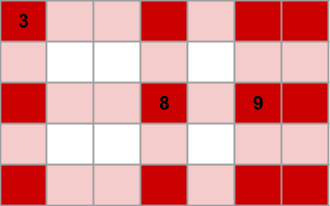
In the depicted input matrix there are 3 fixed cells. The 3 interesting rows and 4 interesting columns are highlighted in light red, and the cells in the intersection of an interesting row and an interesting column are highlighted in dark red. Those dark red cells make up M' and the nodes of G' (besides the root). The fixed cell containing a 3 has two neighbors in G'. The edge going to its vertical neighbor has length 2 × D, because it is 2 steps away in the original M. Similary, the edge going to its horizontal neighbor has length 3 × D.

Having G', we can define p'(c) as the shortest path in G' from the root to each cell c that exists in M'.

Property 5. For each cell c that exists in M', p'(c) = p(c). To prove this, consider a shortest path
root, a₁, a₂, ..., a_k=c
in G from the root to c with the hypothesis of Property 4 (that is, it does horizontal steps first, and vertical steps last). First, notice that if the edge going into a_i is horizontal and the edge going out of it is vertical (that is, a_i is the only corner), then a_i is in M', because it shares a row with a₁, which is a fixed cell and thus it is in M', and a column with a_k=c, which is also in M'. Between a₁ and a_i all moves are horizontal, so we can "skip" the a_js not in M', and the length of the edges in G' will exactly match the sum of the lengths of all intermediate edges. The analogous argument works for all the vertical moves between a_i and a_k.

Notice that Property 5 implies that we can use a similar algorithm over G' to distinguish the impossible cases, as we can calculate p' and then know the value of p'(c) = p(c) for all fixed cells c, which we can use to check Property 2. We still need, however, a way to know the sum over all p(c) for the possible cases, which we can't calculate explicitly.

Let a cell c in M be at row i and column j. Let i₀ be the largest interesting row that is no greater than i, and i₁ be the smallest interesting row that is no less than i. Notice that i₀ = i = i₁ if i is interesting and i₀ < i < i₁ otherwise. Similarly let j₀ and j₁ be the closest interesting columns to j in each direction. We call the up to 4 cells at positions (i₀, j₀), (i₀, j₁), (i₁, j₀) and (i₁, j₁), which are all in M', the sourrounding cells of c.

Property 6. For each non-fixed cell c in row i and column j of M there is a shortest path from the root to c in G that goes through one of its sourrounding cells. This can be proven similarly to Property 4. After the first step of going from the root to the appropriate fixed cell a₁, any path that has the minimum number of horizontal and vertical steps yields the same total length. Notice that there is always a sourrounding cell that is closer to a₁ than c (that's why they are "sourrounding"). Therefore, we can always take a path that goes through that sourrounding cell.

Given Property 6, we can build G', calculate p', and then solve each contiguous submatrix of M delimited by interesting rows as a separate problem. Each of those problems is an instance of our original problem in which we have fixed exactly the four corners. There is overlap in the border among these subproblems, but we can simply subtract the overlapping from the total. Calculating the sum of the overlapping part requires a few of the simple observations required to calculate the problem with four corners fixed, so we concentrate on solving the following: for a given matrix size and values in its 4 corners, calculate its sum (modulo 10⁹+7). It's important not to do modulo while calculating p or p', as that can ruin the calculation because we have inequalities in calculating shortest paths, and inequalities are not preserved under modulo operations. Notice that, if U is an upper bound for the given fixed values for cells, the longest path consists of at most 2 × U steps, so the highest value in the image of p is at most U + 2 × U × D, which is at most U + 2 × U². With U up to 10⁹, that value fits in a 64-bit signed integer, which means we don't need large integers to hold on taking the results modulo 10⁹+7 until the summing part.

Let us call the matrix A and the 4 corners tl, tr, bl and br for top-left, top-right, bottom-left and bottom-right. As we argue in the Small dataset section, each cell's value is determined by one of the fixed cells, in this case, one of the four corners. Given the existence of the shortest path tree, the region of cells that are determined by each given corner (breaking ties by giving an arbitrary priority to corners) is contiguous. For a given corner x and cell c, let us call the influence of x over c i(x,c) to the fixed value x has plus S × D where S is the number of orthogonal steps between x and c. We call lower values of influence stronger. The corner that determines the value of a cell is therefore any of the ones with the strongest influence.

Now, consider the top row: tl has a stronger influence than tr over a left-most contiguous set of cells, and tr has a stronger influence over a right-most set of cells. There may be a single cell where the influence strength is equal. It is not hard to prove that the column at which the strongest influence switches from being tl to tr (if looking from left to right) is the same in this top row as in any other row, because the influence values from tl and tr for the i-th row (from top to bottom) are exactly the same values as the values in the top row plus i × D, so the most influential between tl and tr is always the same across cells in any given column. A similar thing happens with each pair of non-opposite corners. There are 4 such pairs. If we consider the lines that split the influence region of each of those pairs, we have up to 2 vertical and 2 horizontal lines (some of them may overlap), dividing A into up to 9 pieces. All except the middle piece have a single corner that has the most influence, thus they can be solved in the same way.

Consider a matrix of r rows and c columns with a single influential corner with value v. The sum of a row containing the value v is v + (v + D) + (v + 2 × D) + .... This summation can be calculated with a formula. And then, the sum of each other row is c × D larger than the previous one, as we add D to the sum for each column. Again, this yields a summation over a known linear function, which can be reduced by the same known formula.

The middle piece of A has influence from two opposite corners (which pair of opposites depends on the order of the lines). We can again partition A into up to 3 parts: rows with influence from one corner, rows with influence from the other corner, and rows with influence from both. Two of those can be summed with a similar formula as the single influential corner case. The rest is a rectangle partitioned into two stepped shaped pieces where the influence is divided. Those laddered pieces can be summed as the summation over a certain range of a quadratic function, which can also be reduced to a formula.

This finishes the problem. There are lots of technical details, specifically math details, that aren't covered in detail, but we hope this conveys the main ideas. We encourage you to fill in the gaps yourself and ask the community to help out if you can't, as it will be really good practice for your next contest.