Google Code Jam Archive — World Finals 2014 problems
Overview
Gennady Korotkevich is the 2014 Code Jam champion!
The 2014 Google Code Jam World Final was hosted in Los Angeles, and our finalists this year came from all over the world: Belarus, Brazil, Bulgaria, China, Czech Republic, Poland, South Korea, Taiwan, Ukraine, and Russia. We had 26 finalists, including our defending champion Ivan Miatselski (mystic).
There were six problems, and it was extremely challenging to solve them all in the four hours the finalists had. To win the prestigious grand prize, the contestants had to be strategic in deciding which problems they were going to try.
There was a broad range of difficulty in this year’s problems. The small input of Problem B was the easiest, and 25 finalists solved it. Besides that, most finalists managed to solve Problem A and B, as well as the small inputs of Problems C, D, and E. The large inputs of Problems C and D were harder, but were still solved by more than 10 finalists. The large inputs of Problem E and F proved to be the hardest: only our champion solved E, and nobody solved F (though our runner-up came close).
At the end of the round, if we only counted the guaranteed points from small inputs, hos.lyric, eatmore, and mystic would make up the top 3. However, most of the points in a contest like this one come from submissions on large inputs, and eatmore, mystic, and Gennady.Korotkevich had the highest potential number of points. But as we discovered when we unveiled the results of our testing in an increasingly tense room, not all of them got all the points they might have.
The final result: Third place went to China's Yuzhou Gu (sevenkplus), who beautifully solved all problems except for the large input of E, and Problem F. In second place was Russia's Evgeny Kapun (eatmore) whose final attack on the large input of F was not quite correct, but who solved F-small. The winner, with an almost perfect performance on all problems except F was Belarus’s Gennady Korotkevich (Gennady.Korotkevich). This was Gennady's first Code Jam final, but only because he was too young in previous years: he first would have qualified in 2010, at the age of 14. Gennady has earned the title of Code Jam Champion, receiving a prize of $15,000 and a guaranteed ticket to the finals to defend his title next year!
You can see who solved what, when, and how the other contestants fared on the full scoreboard.
This year, we did a live broadcast of the whole contest on YouTube, which you can watch if you have an unusually high level of passion for the subject. It also contains brief explanations of how to solve the problems at the end, in case you're interested in hearing the solutions explained in a different way.
That's it for Google Code Jam 2014! With a record-breaking number of participants and an exciting final, we look forward to seeing you all again soon!
Cast
Problem A. Checkerboard Matrix written by David Arthur. Prepared by John Dethridge and Jonathan Paulson.
Problem B. Power Swapper written by David Arthur. Prepared by Ahmed Aly and Mohammad Kotb.
Problem C. Symmetric Trees written by Steve Thomas. Prepared by John Dethridge and Steve Thomas.
Problem D. Paradox Sort written by David Arthur. Prepared by John Dethridge.
Problem E. Allergy Testing written by Bartholomew Furrow. Prepared by Jonathan Paulson.
Problem F. ARAM written and prepared by Bartholomew Furrow.
Contest analysis presented by Bartholomew Furrow, David Arthur, Denis Savenkov, Felix Halim, Igor Naverniouk, John Dethridge, Jonathan Paulson, Steve Thomas, Steven Zhang, Sumudu Fernando, Topraj Gurung, and Tsung-Hsien Lee.
Solutions and other problem preparation by Ahmed Aly, Alex Fetisov, Bartholomew Furrow, David Arthur, Igor Naverniouk, John Dethridge, Jonathan Paulson, Mohammad Kotb, Petr Mitrichev, Steve Thomas, Sumudu Fernando, and Timothy Loh.
A. Checkerboard Matrix
Problem
When she is bored, Mija sometimes likes to play a game with matrices. She tries to transform one matrix into another with the fewest moves. For Mija, one move is swapping any two rows of the matrix or any two columns of the matrix.
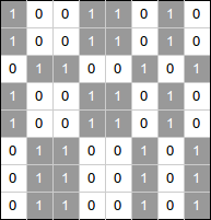
Today, Mija has a very special matrix M. M is a 2N by 2N matrix where every entry is either a 0 or a 1. Mija decides to try and transform M into a checkerboard matrix where the entries alternate between 0 and 1 along each row and column. Can you help Mija find the minimum number of moves to transform M into a checkerboard matrix?
Input
The first line of the input gives the number of test cases, T. T test cases follow. Each test case starts with a line containing a single integer: N. The next 2N lines each contain 2N characters which are the rows of M; each character is a 0 or 1.
Output
For each test case, output one line containing "Case #x: y", where x is the test case number (starting from 1) and y is the minimum number of row swaps and column swaps required to turn M into a checkerboard matrix. If it is impossible to turn M into a checkerboard matrix, y should be "IMPOSSIBLE".
Limits
Memory limit: 1 GB.
1 ≤ T ≤ 100.
Small dataset
Time limit: 60 seconds.
1 ≤ N ≤ 10.
Large dataset
Time limit: 120 seconds.
1 ≤ N ≤ 103.
Sample
3
1
01
10
2
1001
0110
0110
1001
1
00
00
Case #1: 0
Case #2: 2
Case #3: IMPOSSIBLE
In the first sample case, M is already a checkerboard matrix.
In the second sample case, Mija can turn M into a checkerboard matrix by swapping columns 1 and 2 and then swapping rows 1 and 2.
In the third sample case, Mija can never turn M into a checkerboard matrix; it doesn't have enough 1s.
B. Power Swapper
Problem
In a parallel universe, people are crazy about using numbers that are powers of two, and they have defined an exciting sorting strategy for permutations of the numbers from 1 to 2N. They have defined a swapping operation in the following way:
- A range of numbers to be swapped is valid if and only if it is a range of adjacent numbers of size 2k, and its starting position (position of the first element in the range) is a multiple of 2k (where positions are 0-indexed).
- A valid swap operation of size-k is defined by swapping two distinct, valid ranges of numbers, each of size 2k.
To sort the given permutation, you are allowed to use at most one swap operation of each size k, for k in [0, N). Also, note that swapping a range with itself is not allowed.
For example, given the permutation [3, 6, 1, 2, 7, 8, 5, 4] (a permutation of the numbers from 1 to 23), the permutation can be sorted as follows:
- [3, 6, 1, 2, 7, 8, 5, 4]: make a size-2 swap of the ranges [3, 6, 1, 2] and [7, 8, 5, 4].
- [7, 8, 5, 4, 3, 6, 1, 2]: make a size-0 swap of [5] and [3].
- [7, 8, 3, 4, 5, 6, 1, 2]: make a size-1 swap of [7, 8] and [1, 2].
- [1, 2, 3, 4, 5, 6, 7, 8]: done.
Count how many ways there are to sort the given permutation by using the rules above. A way is an ordered sequence of swaps, and two ways are the same only if the sequences are identical.
Input
The first line of the input gives the number of test cases, T. T test cases follow. The first line of each test case contains a single integer N. The following line contains 2N space-separated integers: a permutation of the numbers 1, 2, ..., 2N.
Output
For each test case, output one line containing "Case #x: y", where x is the test case number (starting from 1) and y is the number of ways to sort the given permutation using the rules above.
Limits
Memory limit: 1 GB.
1 ≤ T ≤ 200.
Small dataset
Time limit: 60 seconds.
1 ≤ N ≤ 4.
Large dataset
Time limit: 120 seconds.
1 ≤ N ≤ 12.
Sample
4
1
2 1
2
1 4 3 2
3
7 8 5 6 1 2 4 3
2
4 3 2 1
Case #1: 1
Case #2: 3
Case #3: 6
Case #4: 0
C. Symmetric Trees
Problem
Given a vertex-colored tree with N nodes, can it be drawn in a 2D plane with a line of symmetry?
Formally, a tree is line-symmetric if each vertex can be assigned a location in the 2D plane such that:
- All locations are distinct.
- If vertex vi has color C and coordinates (xi, yi), there must also be a vertex vi' of color C located at (-xi, yi) -- Note if xi is 0, vi and vi' are the same vertex.
- For each edge (vi, vj), there must also exist an edge (vi', vj').
- If edges were represented by straight lines between their end vertices, no two edges would share any points except where adjacent edges touch at their endpoints.
Input
The first line of the input gives the number of test cases, T. T test cases follow.
Each test case starts with a line containing a single integer N, the number of vertices in the tree.
N lines then follow, each containing a single uppercase letter. The i-th line represents the color of the i-th node.
N-1 lines then follow, each line containing two integers i and j (1 ≤ i < j ≤ N). This denotes that the tree has an edge from the i-th vertex to the j-th vertex. The edges will describe a connected tree.
Output
For each test case, output one line containing "Case #x: y", where x is the case number (starting from 1) and y is "SYMMETRIC" if the tree is line-symmetric by the definition above or "NOT SYMMETRIC" if it isn't.
Limits
Memory limit: 1 GB.
1 ≤ T ≤ 100.
Small dataset
Time limit: 60 seconds.
2 ≤ N ≤ 12.
Large dataset
Time limit: 120 seconds.
2 ≤ N ≤ 10000.
Sample
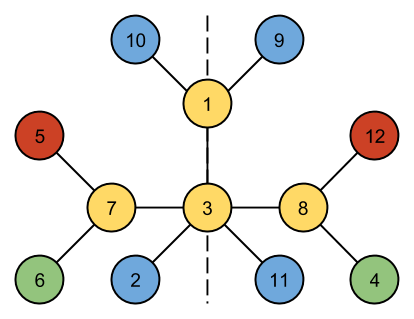
3
4
R
G
B
B
1 2
2 3
2 4
4
R
G
B
Y
1 2
2 3
2 4
12
Y
B
Y
G
R
G
Y
Y
B
B
B
R
1 3
1 9
1 10
2 3
3 7
3 8
3 11
4 8
5 7
6 7
8 12
Case #1: SYMMETRIC
Case #2: NOT SYMMETRIC
Case #3: SYMMETRIC
The first case can be drawn as follows:
No arrangement of the second case has a line of symmetry:
One way of drawing the third case with a symmetry line is as follows:
D. Paradox Sort
Problem
Vlad likes candies. You have a bag of different candies, and you're going to let Vlad keep one of them. You choose an order for the candies, then give them to Vlad one at a time. For each candy Vlad receives (after the first one), he compares the candy he had to the one he was just given, keeps the one he likes more, and throws the other one away.
You would expect that for any order you choose, Vlad will always end up with his favorite candy. But this is not the case! He does not necessarily have a favorite candy. We know for any pair of candies which one he will prefer, but his choices do not necessarily correspond to a simple ranking. He may choose Orange when offered Orange and Lemon, Banana when offered Orange and Banana, and Lemon when offered Lemon and Banana!
There is a particular candy you want Vlad to end up with. Given Vlad's preferences for each pair of candies, determine if there is an ordering such that Vlad will end up with the right candy. If there is, find the lexicographically-smallest such ordering.
Input
The first line of the input gives the number of test cases, T. T test cases follow. Each test case will start with a line containing the integers N and A, separated by a space. N is the number of candies, and A is the number of the candy we want Vlad to finish with. The candies are numbered from 0 to N-1. The next N lines each contains N characters. Character j of line i will be 'Y' if Vlad prefers candy i to candy j, 'N' if Vlad prefers candy j to candy i, and '-' if i = j. Note that if i ≠ j, the jth character of the ith row must be different from the ith character of the jth row.
Output
For each test case output "Case #x: ", where x is the case number, followed by either "IMPOSSIBLE" or a space-separated list of the lexicographically-smallest ordering of candies that leaves Vlad with A.
Limits
Memory limit: 1 GB.
1 ≤ T ≤ 100.
Small dataset
Time limit: 60 seconds.
1 ≤ N ≤ 10.
Large dataset
Time limit: 120 seconds.
1 ≤ N ≤ 100.
Sample
3
2 0
-Y
N-
2 0
-N
Y-
4 3
-YNN
N-YY
YN-Y
YNN-
Case #1: 0 1
Case #2: IMPOSSIBLE
Case #3: 1 2 0 3
E. Allergy Testing
Problem
Kelly is allergic to exactly one of N foods, but she isn't sure which one. So she decides to undergo some experiments to find out.
In each experiment, Kelly picks several foods and eats them all. She waits A days to see if she gets any allergic reactions. If she doesn't, she knows she isn't allergic to any of the foods she ate. If she does get a reaction, she has to wait for it to go away: this takes a total of B days (measured from the moment when she ate the foods).
To simplify her experimentation, Kelly decides to wait until each experiment is finished (after A or B days) before starting the next one. At the start of each experiment, she can choose the set of foods she wants to eat based on the results of previous experiments.
Kelly chooses what foods to eat for each experiment to minimize the worst-case number of days before she knows which of the N foods she is allergic to. How long does it take her in the worst case?
Input
The first line of the input gives the number of test cases, T. T test cases follow. Each test case on a single line, containing three space-separated integers: N, A and B.
Output
For each test case, output one line containing "Case #x: y", where x is the test case number (starting from 1) and y is the number of days it will take for Kelly to find out which food she is allergic to, in the worst case.
Limits
Memory limit: 1 GB.
1 ≤ T ≤ 200.
Small dataset
Time limit: 60 seconds.
1 ≤ N ≤ 1015.
1 ≤ A ≤ B ≤ 100.
Large dataset
Time limit: 120 seconds.
1 ≤ N ≤ 1015.
1 ≤ A ≤ B ≤ 1012.
Sample
3
4 5 7
8 1 1
1 23 32
Case #1: 12
Case #2: 3
Case #3: 0
- First, Kelly eats foods #1 and #2.
- If she gets no reaction after 5 days, she eats food #3. 5 days after that, she will know whether she is allergic to food #3 or food #4.
- If she does get a reaction to the first experiment, then 7 days after the first experiment, she eats food #1. 5 days after that, she will know whether she is allergic to food #1 or food #2.
F. ARAM
Problem
In the game League of Legends™, you can play a type of game called "ARAM", which is short for "All Random, All Mid". This problem uses a similar idea, but doesn't require you to have played League of Legends to understand it.
Every time you start playing an ARAM game, you're assigned one of N "champions", uniformly at random. You're more likely to win with some champions than with others, so if you get unlucky then you might wish you'd been given a different champion. Luckily for you, the game includes a "Reroll" function.
Rerolling randomly reassigns you a champion in a way that will be described below; but you can't reroll whenever you want to. The ability to reroll works like a kind of money. Before you play your first ARAM game, you begin with R RD ("reroll dollars"). You can only reroll if you have at least 1 RD, and you must spend 1 RD to reroll. After every game, you gain 1/G RD (where G is an integer), but you can never have more than R RD: if you have R RD and then play a game, you'll still have R RD after that game.
If you have at least 1RD, and you choose to reroll, you will spend 1RD and be re-assigned one of the N champions, uniformly at random. There's some chance you might get the same champion you had at first. If you don't like the champion you rerolled, and you still have at least 1RD left, you can reroll again. As long as you have at least 1RD left, you can keep rerolling.
For example, if R=2 and G=2, and you use a reroll in your first game, then after your first game you will have 1.5 RD. If you play another game, this time without using a reroll, you will have 2.0 RD. If you play another game without using a reroll, you will still have 2.0 RD (because you can never have more than R=2). If you use two rerolls in your next game, then after that game you will have 0.5 RD.
You will be given the list of champions, and how likely you are to win a game if you play each of them. If you play 10100 games and choose your strategy optimally, what fraction of the games do you expect to win?
Input
The first line of the input gives the number of test cases, T. T test cases follow. Each starts with a line containing three space-separated integers: N, R and G. The next line contains N space-separated, real-valued numbers Pi, indicating the probability that you will win if you play champion i.
Output
For each test case, output one line containing "Case #x: y", where x is the test case number (starting from 1) and y is the proportion of games you will win if you play 10100 games.
y will be considered correct if it is within an absolute or relative error of 10-10 of the correct answer. See the FAQ for an explanation of what that means, and what formats of real numbers we accept.
Limits
Memory limit: 1 GB.
1 ≤ T ≤ 100.
0.0 ≤ Pi ≤ 1.0.
Pi will be expressed as a single digit, followed by a decimal point, followed by 4 digits.
Small dataset
Time limit: 60 seconds.
1 ≤ N ≤ 1000.
1 ≤ R ≤ 2.
1 ≤ G ≤ 3.
Large dataset
Time limit: 120 seconds.
1 ≤ N ≤ 1000.
1 ≤ R ≤ 20.
1 ≤ G ≤ 20.
Sample
3
2 1 1
1.0000 0.0000
3 1 1
1.0000 0.0000 0.5000
6 2 3
0.9000 0.6000 0.5000 0.1000 0.2000 0.8000
Case #1: 0.750000000000
Case #2: 0.666666666667
Case #3: 0.618728522337
Note
League of Legends is a trademark of Riot Games. Riot Games does not endorse and has no involvement with Google Code Jam.
Analysis — A. Checkerboard Matrix
Video of Igor Naverniouk’s explanation.
Let’s start by making some observations about a checkerboard matrix:
- Since a matrix is of dimension 2*N by 2*N, each row and each column have the same number of 0s and 1s.
- Corners of a checkerboard matrix always have two 0s and two 1s, and if we take any submatrix with at least 2 rows and 2 columns (not necessarily square) there will be an even number of 0s and 1s in the corners.
Now, let’s analyze what happens when we swap 2 rows or 2 columns. Such an operation doesn’t change the number of 0s and 1s in a row or column, but more importantly corners of any submatrix will still have even number of 0s and 1s. Indeed, by swapping rows or columns we transform any submatrix with corners located on both of the swapped rows or columns and it will not change the numbers in the corners. This means that any matrix for which the above properties doesn’t hold cannot be transformed into a checkerboard matrix.
Let’s take a matrix for which the above properties hold and consider a pair of rows (the same arguments hold for columns). We can show that all rows that start with 1 will actually be equal to each other and so will be all rows that start with 0 (let’s call these sets of rows A and B). Additionally, corresponding (same column) numbers of a type A and type B row will be different. Thus A rows will be the inverse of B rows. Let’s prove this by considering two rows of the same type. Let’s choose a submatrix with 2 corners fixed in the first column and the others in some other column. By definition of row types, we have 2 corners in the first column equal to each other, but then by the property of a checkerboard matrix we cannot have two different numbers in the other corners as we would get an odd number of 0s or 1s. Therefore, all numbers of same type rows (i.e. A or B) are the same. Analogously we can show that A rows and B rows are the inverse of each other. Since in a checkerboard matrix each row and column has the same number of 0s and 1s, the number of rows of each type is the same. The same arguments hold for columns.
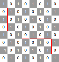
Here is an example of a matrix obtained by permutation of rows and columns of a checkerboard matrix, which demonstrates the facts we just proved:
In a checkerboard matrix, type A and type B rows (and columns) alternate. We note that transformations of rows and columns are independent and we can first find the optimal number of row swaps, then the optimal number of column swaps, and then sum these numbers. Let us denote a type A row (or column) as ‘A’, and a type B row (or column) as ‘B’. Therefore the problem generalizes to the following problem: Given a sequence of 'A' and 'B' characters where the number of ‘A’s is the same as the number of ‘B’s, swap pairs of elements to make the ‘A’s and ‘B’s alternate. We have 2 choices on which letter goes first, either ‘A’ or ‘B’. We can try both. Given the desired order is fixed we can take a pair of ‘A’ and ‘B’ that are in the wrong place and swap them and record the number of swaps.
To conclude, here is the algorithm for the whole problem:
- Start by assigning the first row to type A
-
Go over all rows and compare them element by element with the first row
- if rows equal each other, they are of the same type
- if they are the inverse of each other, they are of type B
- otherwise the given matrix cannot be transformed into a checkerboard matrix and we can output “IMPOSSIBLE”
- Check that the sets A and B have the same number of rows, otherwise output “IMPOSSIBLE”
- The minimum number of row (similarly for column) swaps is equal to min(nswaps_A, nswaps_B) where nswaps_X is the number of wrong positions for type X if we assume that the first row is of type X. The number of wrong positions for type X is equal to the number of rows of type X that reside at even positions. Remember that type A and B must alternate.
- Repeat 1-4 for columns.
- Output the sum of the answers for rows and columns.
Sample implementation in Python 3:
def count_swaps(pos):
  nswaps = 0
  for i in pos:
    if i % 2 == 0:
      nswaps = nswaps + 1
  return nswaps


def inverse(A):
  return [chr(ord('0') + ord('1') - ord(c)) for c in A]

# min_swaps returns minimum swaps required to
# form alternating rows. If B is an invalid matrix,
# returns -1 to denote an impossible case.
def min_swaps(M, N):
  # Step 1.
  typeA = M[0]
  typeB = inverse(typeA)

  pos_A = []
  pos_B = []
  for i in range(2 * N):
    # Step 2 a.
    if M[i] == typeA:
      pos_A.append(i)
    # Step 2 b.
    elif M[i] == typeB:
      pos_B.append(i)
    # Step 2 c.
    else:
      return -1
  # Step 3.
  if len(pos_A) != len(pos_B):
    return -1

  # Step 4.
  return min(count_swaps(pos_A), count_swaps(pos_B))


def solve(M, N):
  # Step 1-4.
  row_swaps = min_swaps(M, N)
  if row_swaps == -1:
    return "IMPOSSIBLE"

  Mt = [list(i) for i in zip(*M)]  # Transpose matrix M

  # Step 5.
  col_swaps = min_swaps(Mt, N)
  if col_swaps == -1:
    return "IMPOSSIBLE"

  return row_swaps + col_swaps


for tc in range(int(input())):
  N = int(input())
  M = []
  for i in range(2 * N):
    M.append(list(input()))
  print("Case #%d: %s" % (tc + 1, solve(M, N)))
Analysis — B. Power Swapper
Video of Bartholomew Furrow’s explanation.
Observe that a swap operation of size 2^x can be performed independently from a swap operation of size 2^y. Thus, we can simplify the sorting process by performing the swaps from the smallest size to the largest size and assume that when performing a swap of size 2^z, the adjacent numbers inside it are fully sorted (by the previous, smaller sized swaps). Fully sorted here means the adjacent numbers are increasing consecutively (i.e., each number is bigger than the previous by 1).
Let’s look at the possible swappings for the smallest 2^k size element where k = 0 (i.e., swapping two sets of size 1). There are 2^N valid sets of size 1. However, we are only interested in swapping two valid sets such that all 2^(k+1) sized valid sets are fully sorted. This is important because when swapping larger sizes, we assume the smaller sized valid sets are all already fully sorted. Let’s look at some examples:
- Permutation: 2 4 1 3. The only way is to swap 2 with 3, yielding 3 4 1 2 where all 2^1 sized valid sets are fully sorted.
- Permutation: 1 4 3 2. There are two ways to perform a swap so that all 2^1 sized valid sets are fully sorted. The first is by swapping 1 with 3 and the other is by swapping 4 with 2.
- Permutation: 1 4 3 2 6 5. In this case, there are 3 valid sets of size 2^1. It needs at least two swaps to make all 2^1 sized valid sets fully sorted. Thus, it is impossible to sort this permutation.
Learning from the examples above, it is sufficient to only consider swapping at most two valid sets of size 2^k for k = 0. We can generalize this for larger k, assuming all valid sets of smaller size are already fully sorted.
To count the number of ways to sort, we can use recursion (backtracking) to simulate all possible swaps. The recursion state contains the underlying array, the value k, and the number of swaps performed so far. The recursion starts from the smallest sized swaps (k = 0) with the original input array, then it decides which valid sets to swap (if any) and recurses to the larger (k + 1) swaps, and so on until it reaches the largest sized swaps (k = N). The depth of the recursion is at most N and there are at most two branches per recursion state (since there are at most two possible swaps for each size) and each state needs O(2^N) to gather at most two valid candidate sets to be swapped. Thus, the algorithm runs in O(2^(N*2)). When the recursion reaches depth N, it has the number of swaps that have been done so far. Since the ordering of the swaps matters, the number of ways is equal to the factorial of the number of swaps. We propagate the number of ways back up to the root to get the final value. Below is a sample implementation in Python 3:
import math

def swap(arr, i, j, sz):  # Swap two sets.
  for k in range(sz):
    t = arr[i + k]
    arr[i + k] = arr[j + k]
    arr[j + k] = t

def count(arr, N, k, nswapped):
  if k == N:
    return math.factorial(nswapped)

  i = 0
  idx = []  # Candidates’ index for swappings.
  sz = 2**k
  while i < 2**N:
    if arr[i] + sz != arr[i + sz]:
      idx.append(i)
    i = i + sz * 2

  ret = 0
  if len(idx) == 0:  # No swap needed.
    ret = count(arr, N, k + 1, nswapped)

  elif len(idx) == 1:  # Only one choice to swap.
    swap(arr, idx[0], idx[0] + sz, sz)
    if arr[idx[0]] + sz == arr[idx[0] + sz]:
      ret = count(arr, N, k + 1, nswapped + 1)
    swap(arr, idx[0], idx[0] + sz, sz)

  elif len(idx) == 2:  # At most 2 choices.
    for i in [idx[0], idx[0] + sz]:
      for j in [idx[1], idx[1] + sz]:
        swap(arr, i, j, sz)
        if arr[idx[0]] + sz == arr[idx[0] + sz]:
          if arr[idx[1]] + sz == arr[idx[1] + sz]:
            ret = ret + count(arr, N, k + 1, nswapped + 1)
        swap(arr, i, j, sz)

  return ret


for tc in range(int(input())):
  N = int(input())
  arr = list(map(int, input().split()))
  print("Case #%d: %d" % (tc+1, count(arr, N, 0, 0)))
Analysis — C. Symmetric Trees
Video of Igor Naverniouk’s explanation.
Given a vertex-colored tree, we want to know whether it is possible to draw the tree in a 2D plane with a line of symmetry (as defined in the problem statement).
An important question to ask is: how many vertices in the tree are located on the symmetry line? We can categorize the answer into two cases. The first is where there is no vertex on the symmetry line, and the second is where there are one or more vertices on the symmetry line. We will discuss each category in the following sections.
No vertex on the symmetry line
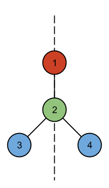
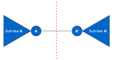
This is the easier case. Since the tree has at least one vertex, there must be a vertex A on the left of the symmetry line connected to another vertex A’ on the right of the symmetry line. The rest of the vertices must belong to the subtree of A or to the subtree of A’. The only edge that crosses the line of symmetry is the edge connecting vertex A and A’. There cannot be any other edges that cross the line of symmetry (otherwise there would be a cycle). The last requirement is that subtree A and subtree A’ are isomorphic. We will elaborate later on how to check whether two subtrees are isomorphic. The following figure illustrates this case:
One or more vertices on the symmetry line
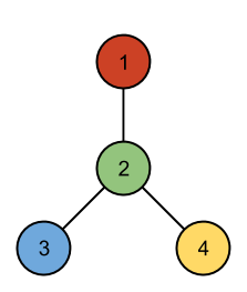
In this case, we can pick a vertex A and put it on the symmetry line. Next, we look at the children of A. Each child represents a subtree. For each child (or subtree) of A we find another (different) child of A that is isomorphic to it. If found, we can put one child on the left side of the symmetry line and the other on the right side of the symmetry line. The root nodes of the subtrees that cannot be paired must be put on the symmetry line. Since there are only two available positions on the line (one is above A and the other is below A), the number of children that cannot be paired must be at most two. These (at most) two children are put on the symmetry line using the same technique described above, except that they can only have one unpaired child (since they have only one available position on the symmetry line). See the following illustration:
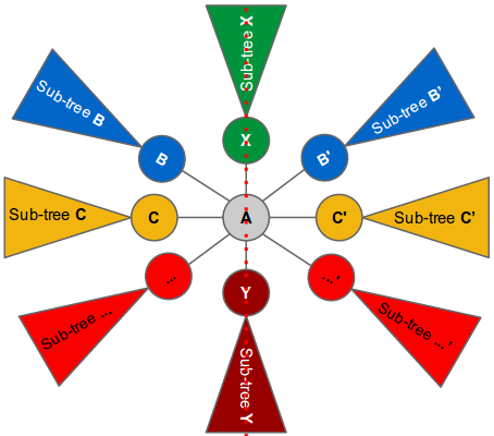
We pair up all children of A that are isomorphic to each other (e.g., B and B’, C and C’ and so on) and put one of them on the left and the other on the right of the symmetry line. There can only be at most two remaining unpaired children (subtree X and subtree Y). We can recursively put X and Y on the symmetry line just above and below vertex A respectively. The subtree of X can only have at most one unpaired child since there is only one available position to put the unpaired child on the symmetry line (i.e., above X). Similarly with the subtree of Y.
How to check whether two subtrees are isomorphic?
The above placing strategies require a quick way of checking whether two subtrees are isomorphic. One way to do this is by encoding each subtree into a unique string representation and then checking whether the strings are equal. One way to encode a subtree into a string is by using a nested-parentheses encoding: starting from the root node of the subtree, construct a string that begins with “(“ followed by the color of the node, then a comma, followed by a sorted, comma-separated list of the encodings of its children (which are computed recursively in the same way), and finally followed by a “)”. For example if node X is the parent of node Y and node Y is the parent of node Z, then the encoding of the subtree X is “(X,(Y,(Z)))”. If node X is the parent of node Z and node Y, then the encoding of the subtree X is “(X,(Y),(Z))”. Note that the children encodings are sorted because we want two subtrees with identical children to produce the same string.
Here is a sample implementation in Python 3:
import sys

def encode_subtree(a, parent):
  children = []
  for b in con[a]:
    if b != parent:
      if con[a][b] == -1:
        con[a][b] = encode_subtree(b, a)
      children.append(con[a][b])

  m = '(' + colors[a]
  for c in sorted(children):
    m += ',' + c
  return m + ')'


def rec_symmetric(a, parent):
  first_pair = {}
  for b in con[a]:
    if b != parent:
      if con[a][b] in first_pair:
        del first_pair[con[a][b]]
      else:
        first_pair[con[a][b]] = b

  keys = list(first_pair.values())
  if len(keys) == 0: return True

  ok = rec_symmetric(keys[0], a)
  if len(keys) == 1 or not ok: return ok

  # Non-root is only allowed one unpaired branch.
  if len(keys) > 2 or parent != -1: return False

  return rec_symmetric(keys[1], a)


def symmetric():
  # No vertex in the middle line.
  for a in range(N):
    for b in con[a]:
      if con[a][b] == con[b][a]:
        return True

  # Pick a vertex in the middle line.
  for a in range(N):
    if rec_symmetric(a, -1):
      return True

  return False


sys.setrecursionlimit(100000)
for tc in range(int(input())):
  colors = []
  con = []

  N = int(input())
  for i in range(N):
    colors.append(input())
    con.append({})

  for i in range(N - 1):
    e = input().split()
    a = int(e[0]) - 1
    b = int(e[1]) - 1
    con[a][b] = -1
    con[b][a] = -1

  for a in range(N):
    encode_subtree(a, -1)

  if symmetric():
    print("Case #%d: SYMMETRIC" % (tc + 1))
  else:
    print("Case #%d: NOT SYMMETRIC" % (tc + 1))
Analysis — D. Paradox Sort
Video of Igor Naverniouk’s explanation.
We can view the set of preferences as a directed graph. We have a node in the graph for each candy, and if we prefer candy X over candy Y, then there is a directed edge from the node for X to the node for Y.
We first describe a procedure to determine if we can find any valid permutation, then we describe a process to find the lexicographically smallest permutation.
Is a permutation possible?
To answer this question, we will use a depth-first search in the graph described above. We use A, the target candy, as the root of the search. A valid permutation exists if and only if we can visit all other candies from the root. Otherwise, there is no valid permutation. Why is that?
If all the candies are reached in the DFS, then we have a directed tree rooted at A containing all the nodes. Then we can generate a valid permutation by printing the nodes using a post-order traversal of the tree (i.e. each node is placed in post-order in the permutation order).
In that permutation, A is the last candy that Vlad will be offered, and Vlad will keep it. To see why this is true, consider the tree implied by the depth-first search. Let X be the candy Vlad is holding before receiving candy A. X must have been preferred to every candy between X and A in the post-order traversal. If X was not a child of A, then one of those candies must be X's parent in the tree, which Vlad would prefer over X. So X must be a child of candy A in the depth-first search, so he will prefer to keep A when offered it.
We demonstrate this with an example for the following test case:
4 1
-YNY
N-YN
YN-N
NYY-
There are 4 candies, and the target candy is candy 1. The candy preferences are shown by directed edges in the figure below. The solid lines represent the tree the DFS found, while the dashed lines represent the edges that were not taken during the DFS.
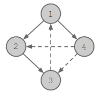
In the post-order traversal, we get the permutation (ordering) 3, 2, 4, 1, which is a valid permutation that leads to our target candy 1 being chosen in the end.
Now we show that if there is a candy that we do not visit in the DFS, then there is no valid permutation. Let X be a candy that is not reached. Let Y be the candy that Vlad keeps after receiving candy X. Y is either X, or another candy which Vlad prefers to X, in which case there is a directed edge in the graph from Y to X. Y is not A, because there cannot be an edge from A to X, or X would have been visited in the depth-first traversal. Consider the list of unique candies that Vlad chooses to keep, in order of time. Assume that Vlad will end up with candy A. The list of kept candies must then end in A, and contain Y earlier in the list. In the sublist of candies between Y and A, Vlad prefers each candy to the one before it. But this means there must be a directed path in the graph from A to X, which is impossible because X was not visited in the DFS. So Vlad cannot end up with candy A.
Thus by using the depth-first traversal procedure, we can answer if the given input can form a valid permutation.
In the following sections, we describe the procedure to generate the lexicographically-smallest permutation.
Checking for valid partial solutions
We will use a greedy strategy to find the lexicographically-smallest permutation. To help us with the greedy strategy, we discuss the case of a partial solution. We want to answer if we can generate a valid permutation from this partial list. In the partial list, the first few numbers (candies) of the lexicographically-smallest permutation have been selected, and one of those candies is the current “best” (preferred) candy B (which might be equal to A). We modify our graph by removing all the numbers (except B) that are already selected in the permutation.
The goal is to answer if we can end up with A from the current partial solution. Trivially, if A is part of the set of removed numbers then it is impossible to generate a valid permutation (we can never end up with A from this state). But if A is not part of the removed set then there are two cases to consider: (i) B is equal to A, or (ii) B is not equal to A. If it is case (i), then A must be preferred over all remaining candies for us to end up with A, otherwise we can report that we cannot generate a valid permutation from this partial solution. Now, let us deal with the more complicated case (ii).
First note that we cannot just use the idea proposed in the section “Is a permutation possible?”, i.e. pick A as the root, then do post-order depth-first traversal on the remaining nodes. The depth-first search might contain a path as follows: A->..->B->Y->Z (see figure below). Then we can't use the post-order traversal, because B is already being held by Vlad, so Y and Z can't occur before it.
Instead, we follow the following procedure:
- Do the same depth-first search, but when visiting B, do not follow any edges out of B.
- Then, for each node X which was not visited by the DFS, and for which there is an edge from B to X, add X as a child of B.
If this succeeds in adding every node to the tree, then it is possible to complete the permutation, otherwise it is not.
To construct the remainder of a permutation from this tree, we first append to the partial solution all the children of B that were added in step 2. Vlad prefers B to each of these. Then we remove B and its children from the tree, and append a post-order traversal of the remaining tree. This results in A winning, for the same reasons as for the algorithm in the previous section for determining feasibility of the whole permutation.
Also similarly to the previous section, we can show that if there is a node X which is not added to the tree by the above procedure, then Vlad cannot be left with A, or else there would be a path from A to X that would have allowed X to be added to the tree.Finding the lexicographically-smallest permutation
We described above a method to determine if we can generate a valid permutation from a given partial solution. Using this idea, we give an algorithm that provides us with the lexicographically-smallest permutation.
We start with an empty prefix of the permutation, then iteratively add the lexicographically smallest candy that leads to a valid prefix. It reports a partial solution as impossible if no candy can be added to the partial solution leading to a valid solution. This algorithm is outlined in the pseudocode below:
Let P = []  // The partial solution

If !IsValidPartialSolution(P)
  return IMPOSSIBLE

Repeat N times
  For i = 1 to N
    // Test if appending i to P gives a valid partial solution
    If P.contains(i) is false
      If IsValidPartialSolution(P + [i]) is true
        P = P + [i]
        Break

Return P
Sample implementation in Python 3:
def dfs(i, removed, visited):
  visited.add(i)
  for j in range(len(prefer[i])):
    if prefer[i][j] == 'Y':
      if j not in visited and j not in removed:
        dfs(j, removed, visited)


def valid(partial):
  B = partial[0]
  for i in partial:
    if prefer[i][B] == 'Y':
      B = i

  removed = set(partial)
  removed.remove(B)

  # Trivial case.
  if A in removed: return False

  # Case (i)
  if A == B:
    for i in range(N):
      if i != A and i not in removed:
        if prefer[A][i] != 'Y':
          return False
    return True

  # Case (ii)
  visited = set([B])
  dfs(A, removed, visited)
  for i in range(len(prefer[B])):
    if prefer[B][i] == 'Y':
      visited.add(i)
  return len(visited.union(removed)) == N


def solve():
  visited = set()
  dfs(A, set(), visited)
  if len(visited) != N: return "IMPOSSIBLE"

  partial = []
  for i in range(N):
    for j in range(N):
      if j not in partial and valid(partial + [j]):
        partial = partial + [j]
        break
  return ' '.join(map(str, partial))


for tc in range(int(input())):
  [N, A] = map(int, input().split())
  prefer = []
  for i in range(N):
    prefer.append(input())
  print("Case #%d: %s" % (tc + 1, solve()))
Analysis — E. Allergy Testing
We describe two solution strategies. First a dynamic programming solution, then a more direct combinatorial solution.
Dynamic programming on the number of foods
At a glance, this sounds like a standard dynamic programming problem where we compute the minimum number of days needed to identify the bad food among the N foods. We can split the N foods into two groups, perform an experiment on one of the groups (i.e., eat all the foods in the first group) and wait for the outcome. If Kelly gets an allergic reaction, then the bad food is in the first group, otherwise it’s in the second group. The number of days needed then depends on the number of days it takes to solve each of the smaller sets.
We can try all possible split sizes for the first group, which gives an O(N^2) solution. We can improve this to O(N) by noticing that the optimal split size for N is always at least as large as the optimal split size for N-1. So we only need to consider split sizes starting at the previous split size, and in total only O(N) split positions are considered. Looking at the constraints for the small input, where N can be as large as 10^15, it is obvious that this is not the way to go. However, this approach may give some insight on how to improve the solution (as we shall see in the next section).
You may wonder why splitting the N foods equally and performing experiments on one of the groups does not give an optimal answer. Consider an example where A = 1, B = 100, and N = 4. In this case, the cost of having an allergic reaction is very high. It is better to perform an experiment one food at a time because as soon as Kelly eats the bad food, she will know about it the next day and thus the whole process only takes at most 3 days. But if she splits into two groups of size 2 and performs an experiment on one of the groups, she risks getting an allergic reaction and still being unable to identify the bad food and will have to wait 100 days for the next experiment. Therefore splitting the N foods equally may not lead to an optimal solution.
Dynamic programming on the number of days
After playing around with some small cases where A and B are at most 100, you will discover that the minimum number of days needed is only in the range of thousands, even for large N. This gives a hint that using the number of days as the DP state could be much more efficient. We can use DP to compute max_foods(D), the maximum number of foods for which Kelly can identify the bad food using at most D days. If we can compute max_foods(D) quickly, we can compute the final answer by finding the smallest X where max_foods(X) >= N.
To compute max_foods(D), we are going to construct a full binary tree that represents a strategy that handles the largest possible number of foods in at most D time. Each node in the tree corresponds to a set of foods. Kelly starts at the root node, and performs a series of tests. Each test narrows down the set of foods, and she moves to the node corresponding to that set. To do this, she eats all the foods in the right child of the current node. If she does not get a reaction, she moves to the left child. If she does get a reaction, she moves to the right child. Leaf nodes of the tree correspond to single foods. When Kelly reaches a leaf node, she has figured out the food to which she is allergic, and can stop.
Define the "height" of a node to be the number of days remaining at that node. The root node has height D, and each other node must have height at least 0. If a node has height X, then its left child has height X-A, since it takes A days until Kelly knows she has not had a reaction. Its right child has height X-A if it is a leaf, and X-B otherwise. This is because Kelly only has to wait B days if she needs to perform another test when the reaction has worn off.
Define the "value" of a node to be the size of the set of foods to which that node corresponds.
Let’s look at an example of a node with height = D and value = max_foods(D) = max_foods(D-A) + max_foods(D-B):
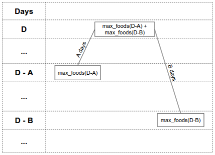
The height of the left child is D - A days, and it has value max_foods(D - A). The height of the right child is D - B days, and it has value max_foods(D - B). This means that if Kelly has a budget of D days and max_foods(D - A) + max_foods(D - B) foods to be processed, she can divide the foods into two groups: the first group is of size max_foods(D - A) foods and the second group is of size max_foods(D - B) foods.
If the tree corresponds to a strategy for handling max_foods(D) foods, then each subtree must contain as many nodes as possible given the time constraints, otherwise we could produce a better strategy by changing that subtree.
So if more than one food can be handled at a node A, then its value must be max_foods(height(A)).
The situation for leaf nodes, where only one food can be handled, is more complex. If the node is the left child of its parent, then its height must be less than A, otherwise we could handle at least two foods there instead. If the node is the right child of its parent, then its height must only be less than B. This is because if another food is added, then Kelly must wait B days after the previous test instead of A days.
Let’s see an example where we want to compute max_foods(8) where A = 2 and B = 3. We can construct the following full binary tree:
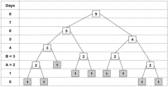
The root node has height = 8 days. Using the rules described above, we can continue traversing the children until we reach the leaf nodes. Going up from the leaf nodes all the way to the root, we can compute the value of the intermediate nodes by summing the value of their two children. From the figure above, we can figure out that max_foods(8) = 9, and similarly max_foods(6) = 5, max_foods(5) = 4, etc.
Nodes with the same height always have the same value (except for the case of leaves which are right children.)
Thus, we can use memoization to do the computation in O(days needed). Here is a sample implementation in Python 3:
from functools import lru_cache

@lru_cache(maxsize = None)  # Memoization.
def max_foods(D, A, B):
  if D < A: return 1  # Leaf node.
  return max_foods(D - A, A, B) + max_foods(D - B, A, B)

# We can also use binary search here.
def min_days(N, A, B):
  days = 0
  while max_foods(days, A, B) < N:
    days = days + 1
  return days

for tc in range(int(input())):
  print("Case #%d: %d" % (tc+1, \
    min_days(*map(int, input().split()))))
The above solution assumes that the answer (i.e., the number of days) is limited to a few thousand days, which is true for the small input cases where A and B is at most 100. For the large input cases, A and B can be up to 10^12 which makes the above solution infeasible.
Dynamic programming on the number of edges of each type
Observe that for large A and B, the set of days D where max_foods(D) is larger than max_foods(D-1) is sparse. Each edge reduces the remaining time by either A or B. Call these A-edges and B-edges. Since the height of a node depends only on the number of A-edges and B-edges on its path to the root, we can use a more “compact” DP state to compute max_foods(D) by using the number of A-edges and B-edges instead of using the height as shown in the sample implementation in Python 3 below:
INF = 1e16

def max_foods(D, A, B):
  ans = 0
  mem = [0] * 60  # zero-array of 60 elements.
  mem[0] = 1
  for i in range(int(D / A + 1)):  # A-edges.
    for j in range(int(D / B + 1)):  # B-edges.
      H = i * A + j * B  # Height of this node.

      # Skip this node if it uses more than D days.
      if H > D: break

      # Aggregate the child’s value.
      if j > 0 and H + A <= D: mem[j] += mem[j-1]

      # if we are too close to D to add a B-edge,
      # the right child is a leaf,
      # so add this node to the answer.
      if H + B + A > D: ans += mem[j]

      # Avoid overflows.
      ans = min(ans, INF)
      mem[j] = min(mem[j], INF)

  return ans
Notice that the above code reuses the DP array as it iterates through the A-edges, and the number of B-edges is limited to < 60, so the memory footprint is very small. However, this approach does not work when the number of A-edges is very large. This number can be as large as 50 * B / A, so whether this solution works depends closely on the ratio B / A. In the next two sections we provide two solutions to address this issue.
Solution 1: Use a closed-form solution for #B-edges <= 2.
Observe that as the ratio B / A gets large, the number of B-edges in the solution ends up being very small and the number of A-edges ends up being very large (which makes the dynamic programming solution above run very slow). In fact, if B / A > N, then the solution will involve no B-edges at all. This corresponds to a strategy of trying the foods one at a time until you find the correct one. It is possible to derive closed forms to compute max_foods(D) if there are at most 0, 1 and 2 B-edges in the solution, corresponding to tree heights <B+A, <2B+A and <3B+A respectively. For a ratio B / A greater than 200,000, the maximum tree height is less than 3B+A and so we can get the solution from one of these closed forms. If the ratio is less than 200,000, we can fall back to our dynamic programming solution.
Below is the sample implementation in Python 3 of the closed form solutions for computing max_foods(D) where there are at most 0 (linear), 1 (quadratic), or 2 (cubic) B-edges:
def linear(D, A, B):
  return int(D / A + 1)

def quadratic(D, A, B):
  R = int((D - B) / A)
  if INF / R < R: return INF
  return int(linear(D, A, B) + (R * (R + 1)) / 2)

def cubic(D, A, B):
  ans = quadratic(D, A, B)
  a = int((D - 2 * B) / A)
  for i in range(a):
    R = a - i
    if INF / R < R: return INF
    ans += int((R * (R + 1)) / 2)
    if ans > INF: return INF
  return ans
To put it all together, we can determine which closed form solution to use, or use the compact dynamic programming as the fallback and then use binary search to find the minimum days needed. Here is the rest of the code:
def binary_search(N, A, B, low, high, func):
  while high - low > 1:
    D = int((high + low) / 2)
    if func(D, A, B) >= N:
      high = D
    else:
      low = D
  return high

def min_days(N, A, B):
  if quadratic(B + A, A, B) >= N:
    return binary_search(N, A, B, -1, B + A, linear)
  if cubic(2 * B + A, A, B) >= N:
    return binary_search(N, A, B, B + A, 2 * B + A, quadratic)
  if cubic(3 * B + A, A, B) + 1 >= N:
    return binary_search(N, A, B, 2 * B + A, 3 * B + A, cubic)
  return binary_search(N, A, B, 3 * B + A, 51 * B, max_foods)

for tc in range(int(input())):
  print("Case #%d: %d" % (tc+1, \
    min_days(*map(int, input().split()))))
Solution 2: Speed up the dynamic programming solution through fast matrix exponentiation
There is another way to handle very large number of A-edges without using closed form formulae. Observe that in the dynamic programming solution code, the mem vector at stage i+1 is a linear sum of itself at stage i, so we can represent the transition as a matrix-vector multiplication, implementing the answer as an accumulator parameter in the vector. We can therefore accelerate the process using fast matrix exponentiation.
There is a slight complication in that the matrix is not the same for all i. If p_j is the smallest index j for which H + A > D, then the matrix describing the state transition remains constant as long as p_j doesn't change. However, we can see from the structure that p_j is monotonically decreasing with increasing i and it can therefore only take 50 different values at most. We can therefore break up the computation into at most 50 ranges of continuous p_j and perform our matrix exponentiation to get the answer to each of them.
The complexity of this method could be as high as log^6 N, from factors log N for the binary search, log N ranges of p_j, matrix multiplications of log^3 N and log N for the fast exponentiation. However, not all of these parameters can be large simultaneously and it's likely that the actual time bound is somewhat tighter than this coarse estimate.
Combinatorial solution
We can compute max_foods(T) more directly, and then do a binary search to find the minimum T such that max_foods(T) >= N.
For each leaf, we write down a string of 'x' and 'y' characters that indicates the path taken from the root to the leaf. 'x' indicates a left branch, and 'y' indicates a right branch. For paths that end with a right branch, and have height < B-A, remove the final 'y'.
Each leaf's string now consists of some unique arrangement of K 'x' characters and L 'y' characters, where T-B < KA + LB <= T. Also, each possible string of 'x' and 'y' characters satisfying the above constraint corresponds to a leaf in the tree. We can determine the number of leaves by counting the number of these strings. There are (K+L) choose L strings that contain 'x' K times and 'y' L times. So, we have:
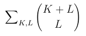
where T-B < KA + LB <= T
We can easily compute the minimum and maximum K such that T-B< KA+LB <= T for a given L. So we can rewrite the sum above as:
Which equals:
Since the number of strings grows exponentially with L, the maximum L is O(log N), so we can compute this sum efficiently.
Below is a sample implementation in Python 3. Note that Python has a built in big integer, thus we don’t need to worry so much about overflow.
def nCk(n, k):
  if k > n: return 0
  res = 1
  for i in range(1, min(n - k, k) + 1):
    res = res * (n - i + 1) // i
  return res

def max_foods(D, A, B):
  cnt = 0
  for L in range(min(51, D // B + 1)):
    K_min = (D - L * B - B) // A + 1
    K_max = (D - L * B) // A
    cnt += nCk(K_max + L + 1, L + 1) - nCk(K_min + L, L + 1)
  return cnt

def min_days(N, A, B):
  lo = 0
  hi = int(1e15)
  while lo < hi:
    D = (lo + hi) // 2
    if max_foods(D, A, B) >= N:
      hi = D
    else:
      lo = D + 1
  return lo

for tc in range(int(input())):
  print("Case #%d: %d" % (tc+1, \
    min_days(*map(int, input().split()))))
Analysis — F. ARAM
We are going to do a binary search to find the answer. At each iteration of the binary search, we have some estimate of the answer Q, and we need to decide if that estimate is too high or too low. We do this by trying to find a strategy that can achieve a fraction Q of wins in the long run.
We need to describe what a valid strategy is. In a straightforward dynamic programming formulation of the problem, the current state would be the champion we have been assigned, the amount of money we have, and the number of games that remain; the decision we would need to make at each state is whether to reroll.
Obviously we cannot compute the decision for each of these states individually; there are O(10^100 * N * R * G) of them! But since the number of games that will be played is immense, we can assume that the number of games remaining is unimportant, and just optimize assuming there are "infinite" games remaining. It can be proved that the amount of error this will induce in the answer is far less than 10^-10, the required precision. Also note that if we reroll when assigned a certain champion for a particular amount of money, then it also makes sense to reroll when assigned a champion with a lower winning probability, with the same amount of money. So to compute a strategy, we we only need to decide for each amount of money, which hero we would reroll that has the highest winning probability.
But how do we evaluate how good a strategy is, when we're going to play infinite games? When we are low on money, we need to be more conservative about when we reroll. If we reroll too aggressively when we have very little money left and our amount of money drops below 1 dollar, we will not be able to reroll for a while and our expected number of wins will drop. Intuitively what we need to determine is, if our money gets low, to say M dollars, how much will we fall behind our expected number of won games before our amount of money improves to M+1/G?
We define the "surplus" for a set of games as the number of games won in the set minus Q multiplied by the number of games played in the set. We choose our strategy at M money to maximize the expected surplus of the set of games that occur until we reach M+1/G money. (If M is equal to R, then our amount of money will not increase, so we use the set of games that lasts until we have M money again.) Let this value be A[M].
If M<1 then we cannot reroll, so
since the set will consist of exactly one game, and we get a random champion.
For 1 <= M < R, suppose that our strategy requires that we will reroll the worst K_M heroes. Sort the values Pi. Then:

Similarly, for M=R:
We can compute the optimal values for A by optimizing for K_M separately for each M from 0 to R. Note that A[M]>=-1 for all M, since the strategy of never rerolling has a surplus no worse than -1, so the optimal strategy must be at least as good as that.
If A[R]>=0, we decide that Q is too high. If A[R]<0, we decide that Q is too low. We now show that this works.
We start with R money. We will return to R money multiple times, with expected surplus A[R] each time, until finally we reach 10^100 games and stop. Consider instead the scenario where once we reach 10^100 games, we keep playing until we reach R money again. The expected surplus in this scenario is T*A[R], where T>=1 is the expected number of times we return to R money. Now, let X be the expected surplus of the games after the 10^100th. From the definition of A, X=A[M] + A[M+1/G] + ... + A[R-1/G], where M is the amount of money we have after game 10^100.
Assume that A[M]<0 for M<R (if not, we can play as if R was equal to the lowest M such that A[M] >= 0 and the proof will work). Then -RG <= X < 0.
Now the surplus for the first 10^100 games is Y=T*A[R] - X. Therefore T*A[R] < Y <= T*A[R] + RG.
RG is insignificant over 10^100 games. So the fraction of expected wins for this strategy is Q + T*A[R] * 10^-100. So we assert that if A[R] >= 0, then we can achieve a strategy which wins a fraction of at least Q, and otherwise we cannot. This will allow our binary search to converge to a sufficiently accurate answer.
Below is a sample implementation in Python 3. To avoid fractional dollars, we introduce a smaller unit (e.g., a coin) C for the money where G coins is equal to one dollar.
# Can you win at least X fraction of the time?
def CanWin(X):
  A = []
  last_G_values = 0

  # C < G, not enough coins for a reroll.
  for C in range(0, G):
    A.append(avg_win_prob_top[N] - X)
    last_G_values += A[C]

  # C >= G, enough coins for a reroll.
  for C in range(G, R * G + 1):
    A.append(-1e100)
    for K in range(1, N + 1):
      p = (N - K) / N  # Probability of rerolling.
      p_reroll = p / (1 - p) * last_G_values
      p_not_reroll = avg_win_prob_top[K] - X
      A[C] = max(A[C], p_reroll + p_not_reroll)

    if A[C] >= 0: return True
    last_G_values += A[C] - A[C - G]

  return False


for tc in range(int(input())):
  [N, R, G] = map(int, input().split())
  win_prob = map(float, input().split())
  win_prob = sorted(win_prob, reverse=True)

  avg_win_prob_top = [0]
  for topK in range(1, N + 1):
    avg_win_prob_top.append(sum(win_prob[0:topK]) / topK)

  lo = 0
  hi = 1
  for i in range(60):
    mid = (lo + hi) / 2
    if CanWin(mid):
      lo = mid
    else:
      hi = mid

  print("Case #%d: %.15f" % (tc + 1, lo))
An alternative solution is to evaluate strategies by modelling the game as a Markov chain and computing its stationary distribution, then iteratively improving the strategy. It is quite difficult to do this with sufficient accuracy.