Google Code Jam Archive — Round 2 2014 problems
Overview
This round was very challenging. Problem A was solved very quickly in just 4:21 minutes, and a lot of people ended up solving the first two problems, Burunduk1 solved the two in just 9:31 minutes. After the solutions for problem A and problem B, the rate of solutions decreased and most of the contestants decided to solve the small input files for problem C and problem D using brute-force approaches instead of efficient methods required for to solve the large-input.
Gennady.Korotkevich got first place with a full score and a time penalty of 1:06:38 (which with a 4-minute penalty ended up being a time penalty of 1:10:38), while yeputons got second place and was just 1:11 minutes behind Gennady. All in all, 37 contestants were able to get the full score!
Note that to quality for Round 3, it was sufficient to solve problem A, problem B, problem C’s small-input, and problem D’s small-input in 2:27:18 hours or less.
Congratulations to the Top 500 who qualified to advance to Round 3, and the Top 1000 who got a T-shirt!
Cast
Problem A. Data Packing written by Khaled Hafez. Prepared by Mohammad Kotb.
Problem B. Up and Down written by David Arthur. Prepared by Jonathan Paulson and Mohammad Kotb.
Problem C. Don't Break the Nile written and prepared by Jonathan Wills.
Problem D. Trie Sharding written by David Arthur. Prepared by Jonathan Paulson and Igor Naverniouk.
Contest analysis presented by David Arthur, Felix Halim, Igor Naverniouk, Mohammad Kotb, Topraj Gurung, and Zong-Sian Li.
Solutions and other problem preparation by Ahmed Aly, Bartholomew Furrow, Carlos Guía, John Dethridge, Jonathan Shen, Momchil Ivanov, Sumudu Fernando, Onufry Wojtaszczyk, Patrick Nguyen, Petr Mitrichev, and Tiancheng Lou.
A. Data Packing
Problem
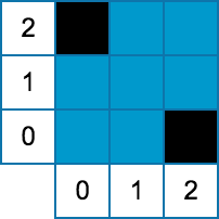
Adam, being a well-organized man, has always been keenly interested in organizing all his stuff. In particular, he fondly remembers the many hours of his youth that were spent moving files from his computer onto Compact Discs.
There were two very important rules involved in this procedure. First, in order to ensure that all discs could be labeled clearly, Adam would never place more than two files on the same disc. Second, he would never divide a single file over multiple discs. Happily, the discs he was using were always large enough to make this possible.
Thinking back, Adam is now wondering whether he arranged his files in the best way, or whether he ended up wasting some Compact Discs. He will provide you with the capacity of the discs he used (all his discs had the same capacity) as well as a list of the sizes of the files that he stored. Please help Adam out by determining the minimum number of discs needed to store all his files—following the two very important rules, of course.
Input
The first line of the input gives the number of test cases, T. T test cases follow. Each test case begins with a line containing two integers: the number of files to be stored N, and the capacity of the discs to be used X (in MBs). The next line contains the N integers representing the sizes of the files Si (in MBs), separated by single spaces.
Output
For each test case, output one line containing "Case #x: y", where x is the case number (starting from 1) and y is the minimum number of discs needed to store the given files.
Limits
Memory limit: 1 GB.
1 ≤ T ≤ 100.
1 ≤ X ≤ 700.
1 ≤ Si ≤ X.
Small dataset
Time limit: 60 seconds.
1 ≤ N ≤ 10.
Large dataset
Time limit: 120 seconds.
1 ≤ N ≤ 104
Sample
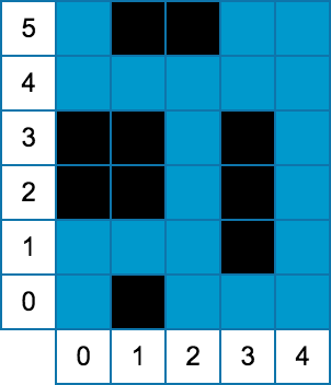
3
3 100
10 20 70
4 100
30 40 60 70
5 100
10 20 30 40 60
Case #1: 2
Case #2: 2
Case #3: 3
B. Up and Down
Problem
You are given a sequence of distinct integers A = [A1, A2, ..., AN], and would like to rearrange it into an up and down sequence (one where A1 < A2 < ... < Am > Am+1 > ... > AN for some index m, with m between 1 and N inclusive).
The rearrangement is accomplished by swapping two adjacent elements of the sequence at a time. Predictably, you are particularly interested in the minimum number of such swaps needed to reach an up and down sequence.
Input
The first line of the input gives the number of test cases, T. T test cases follow. Each test case begins with a line containing a single integer: N. The next line contains N distinct integers: A1, ..., AN.
Output
For each test case, output one line containing "Case #x: y", where x is the test case number (starting from 1) and y is the minimum number of swaps required to rearrange A into an up and down sequence.
Limits
Memory limit: 1 GB.
1 ≤ T ≤ 100.
1 ≤ Ai ≤ 109
The Ai will be pairwise distinct.
Small dataset
Time limit: 60 seconds.
1 ≤ N ≤ 10.
Large dataset
Time limit: 120 seconds.
1 ≤ N ≤ 1000.
Sample
2
3
1 2 3
5
1 8 10 3 7
Case #1: 0
Case #2: 1
In the first case, the sequence is already in the desired form (with m=N=3) so no swaps are required.
In the second case, swapping 3 and 7 produces an up and down sequence (with m=3).
C. Don't Break The Nile
Problem
Aliens have landed. These aliens find our Earth's rivers intriguing because their home planet has no flowing water at all, and now they want to construct their alien buildings in some of Earth's rivers. You have been tasked with making sure their buildings do not obstruct the flow of these rivers too much, which would cause serious problems. In particular, you need to determine what the maximum flow that the river can sustain is, given the placement of buildings.
The aliens prefer to construct their buildings on stretches of river that are straight and have uniform width. Thus you decide to model the river as a rectangular grid, where each cell has integer coordinates (X, Y; 0 ≤ X < W and 0 ≤ Y < H). Each cell can sustain a flow of 1 unit through it, and the water can flow between edge-adjacent cells. All the cells on the south side of the river (that is with y-coordinate equal to 0) have an implicit incoming flow of 1. All buildings are rectangular and are grid-aligned. The cells that lie under a building cannot sustain any flow. Given these constraints, determine the maximum amount of flow that can reach the cells on the north side of the river (that is with y-coordinate equal to H-1).
Input
The first line of the input gives the number of test cases, T. T test cases follow. Each test case will begin with a single line containing three integers, W, the width of the river, H, the height of the river, and B, the number of buildings being placed in the river. The next B lines will each contain four integers, X0, Y0, X1, and Y1. X0, Y0 are the coordinates of the lower-left corner of the building, and X1, Y1 are the coordinates of the upper-right corner of the building. Buildings will not overlap, although two buildings can share an edge.
Output
For each test case, output one line containing "Case #x: m", where x is the test case number (starting from 1) and m is the maximum flow that can pass through the river.
Limits
Memory limit: 1 GB.
1 ≤ T ≤ 100.
0 ≤ X0 ≤ X1 < W.
0 ≤ Y0 ≤ Y1 < H.
Small dataset
Time limit: 60 seconds.
3 ≤ W ≤ 100.
3 ≤ H ≤ 500.
0 ≤ B ≤ 10.
Large dataset
Time limit: 120 seconds.
3 ≤ W ≤ 1000.
3 ≤ H ≤ 108.
0 ≤ B ≤ 1000.
Sample
2
3 3 2
2 0 2 0
0 2 0 2
5 6 4
1 0 1 0
3 1 3 3
0 2 1 3
1 5 2 5
Case #1: 1
Case #2: 2
|
|
D. Trie Sharding
Problem
A set of strings S can be stored efficiently in a trie. A trie is a rooted tree that has one node for every prefix of every string in S, without duplicates.
For example, if S were "AAA", "AAB", "AB", "B", the corresponding trie would contain 7 nodes corresponding to the prefixes "", "A", "AA", AAA", "AAB", "AB", and "B".
I have a server that contains S in one big trie. Unfortunately, S has become very large, and I am having trouble fitting everything in memory on one server. To solve this problem, I want to switch to storing S across N separate servers. Specifically, S will be divided up into disjoint, non-empty subsets T1, T2, ..., TN, and on each server i, I will build a trie containing just the strings in Ti. The downside of this approach is the total number of nodes across all N tries may go up. To make things worse, I can't control how the set of strings is divided up!
For example, suppose "AAA", "AAB", "AB", "B" are split into two servers, one containing "AAA" and "B", and the other containing "AAB", "AB". Then the trie on the first server would need 5 nodes ("", "A", "AA", "AAA", "B"), and the trie on the second server would also need 5 nodes ("", "A", "AA", "AAB", "AB"). In this case, I will need 10 nodes altogether across the two servers, as opposed to the 7 nodes I would need if I could put everything on just one server.
Given an assignment of strings to N servers, I want to compute the worst-case total number of nodes across all servers, and how likely it is to happen. I can then decide if my plan is good or too risky.
Given S and N, what is the largest number of nodes that I might end up with? Additionally, how many ways are there of choosing T1, T2, ..., TN for which the number of nodes is maximum? Note that the N servers are different -- if a string appears in Ti in one arrangement and in Tj (
Input
The first line of the input gives the number of test cases, T. T test cases follow. Each test case starts with a line containing two space-separated integers: M and N. M lines follow, each containing one string in S.
Output
For each test case, output one line containing "Case #i: X Y", where i is the case number (starting from 1), X is the worst-case number of nodes in all the tries combined, and Y is the number of ways (modulo 1,000,000,007) to assign strings to servers such that the number of nodes in all N servers are X.
Limits
Memory limit: 1 GB.
1 ≤ T ≤ 100.
Strings in S will contain only upper case English letters.
The strings in S will all be distinct.
N ≤ M
Small dataset
Time limit: 60 seconds.
1 ≤ M ≤ 8
1 ≤ N ≤ 4
Each string in S will have between 1 and 10 characters, inclusive.
Large dataset
Time limit: 120 seconds.
1 ≤ M ≤ 1000
1 ≤ N ≤ 100
Each string in S will have between 1 and 100 characters, inclusive.
Sample
2
4 2
AAA
AAB
AB
B
5 2
A
B
C
D
E
Case #1: 10 8
Case #2: 7 30
Analysis — A. Data Packing
Given a list of file sizes, Adam wants to pack these files in the minimum number of compact discs where each disc can fit upto 2 files and a single file cannot be divided into multiple discs. All compact discs have the same capacity X MB.
There are several greedy approaches that can solve this problem. We describe one and show how it can be implemented efficiently. We first sort all file sizes. Then we linearly scan the sorted list going from smallest to biggest. For each file, we try to “pair” it with the largest possible file that can both fit in X. If no such largest file is found, we put the file by itself. We finally report the number of discs used.
Let’s analyze the running time for this solution. The sorting take O(N log N), and the linear scan combined with searching for largest possible file take O(N2). Therefore the running time for this algorithm is O(N2) which is sufficient to solve the large data set.
We can further optimize this solution by avoiding the O(N2) computation. To do so, we use a common idea used in programming competitions. First, as before, we sort the file sizes. We then keep track of two pointers (or indices) A and B: A initially points to the smallest index (i.e., index 0), and B initially points to the largest index (i.e., index N-1). The idea being that at any instance, the two pointers A and B point to two candidate files that can be paired and placed in one disc. If their combined size fits in X, then we place it in one disc and then “advance” both pointers simultaneously, i.e. we increase A by 1, and decrease B by 1. If the combined file size does not fit in X, then we repeat the process of decreasing B by 1 -- which means the large disc which was previously at index B will need to be put in a disc by itself -- until the combined file size at A and B fits in X. During this iteration, we should handle the case when A and B point to the same index i.e. ensure we do not double count that file. After a matching file has been found at B, we simultaneously advance A and B as before. We should repeat this process only when B is greater than or equal to A. As for the running time, advancing the largest and smallest pointers takes O(N) time, therefore the running time is dominated by sorting which is O(N log N).
As an aside, we would like to point out that for the first solution sorting isn’t actually necessary. We can instead pick any file, then find the largest file that fits with it in a disc. If no such largest file exists, we can put the file by itself. Intuitively, the reason why it works is because we greedily try to “pair” each file with the best possible largest file. This algorithm still has a O(N2) running time.
Analysis — B. Up and Down
Given a sequence of distinct numbers, we are asked to rearrange it by using a series of swaps of adjacent elements resulting in an up and down sequence. We want to do it in such a way that the total number of swaps is minimized.
We describe a greedy solution. We use the example sequence 6,5,1,4,2,3 to help explain the solution.
- Repeat N times:
- Pick the smallest value in the sequence. In the example sequence, it is 1.
- Determine if the smallest value is closer to the left end of the sequence or the right end of the sequence. In the example, the left end is where 6 is and the right end is where 3 is. The smallest value, 1 is closer to the left end (2 swaps away) than the right end (3 swaps away).
- Move the smallest value towards the closest end by swapping with adjacent elements, and record the number of swaps. In the example, we move 1 towards 6, first swapping 1 and 5, then swapping 1 and 6 resulting in the sequence: 1,6,5,4,2,3. We performed 2 swaps.
- Remove the smallest number from the sequence. In the example, we remove 1 resulting in the sequence 6,5,4,2,3.
- Repeat the process on the resulting sequence. In our example, we repeat the process on sequence 6,5,4,2,3. We identify the smallest element, which is 2, then move it towards the closer end which is the right end with 1 swap, then remove 2 resulting in sequence 6,5,4,3. We then repeat the process on this sequence. First pick smallest value which is 3. Since 3 is already on the right most end, we perform 0 swaps to move it to the closer end, then we remove 3. We repeat a similar process for values 4, 5, then finally 6.
- Finally, report the total number of swaps. In our example, we performed 2 + 1 = 3 swaps.
That’s it! You might be wondering why the greedy algorithm works. We provide an intuition here. At each step in our algorithm, we pick the smallest number. In the final up and down sequence, this smallest number will need to go to one of the ends at some point in time. We move this smallest number to the closer end to minimize the number of swaps. After this smallest number reaches the closer end, its position is final, i.e. its position in the final up and down sequence is set, therefore it will never need to be moved/swapped further. Thus, in the next step we can remove that smallest number from consideration and work on a completely new sequence that is one size smaller. We repeat the process for this new sequence, i.e. move the smallest element to the closer end, then remove that number, until we reach the empty sequence. Since we perform the minimum number of swaps in each step on each sub-problem (sequence which is 1 size smaller), we minimize the number of swaps for the whole problem.
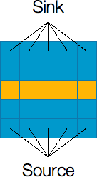
Analysis — C. Don't Break The Nile
We are given a grid (representing a river) of size W x H filled with disjoint rectangles (representing buildings). Each cell in the grid that is not covered by a rectangle can sustain a flow of 1 unit of water through it and the water can flow to edge-adjacent cells. Cells that are covered by a rectangle cannot sustain any flow. All cells at the bottom (south side) have an implicit incoming flow of 1 unit. You are to find the maximum unit of water that can flow to the cells at the top (north side).
A Greedy Approach
If we consider a "stream" of water being a one unit connected path from the bottom to the top, then the problem can be considered as finding the maximum number of disjoint streams that can fit within the grid. If we had to find one valid stream at a time, then it would make the most sense to try to keep the stream as close to a boundary of the board as possible, because that leaves the most spaces available for future streams.
Taking this idea into an algorithm, we can start at the bottom-left-most available square, and use the left-hand-rule described here. We essentially walk forward with the goal of reaching the top, keeping as close to the left wall as possible. We show this idea in the example below. The figure shows the buildings in black, and the other colored (i.e., red, green, yellow, blue, and magenta) portions are the river. To help visualize the left-hand-rule walk, we can imagine an infinite wall on the left and right side of the river.
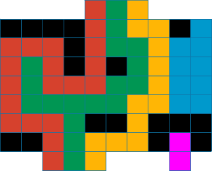
The first stream starts from the bottom-left-most available square which is on the 3rd cell from the left (colored red). The path to the top keeps as close to the left wall as possible as shown by the red colored cells. The second stream is the green colored cells. It goes upwards, to the left and back (since it is a dead-end) and continues to the right, keeping as close to the left wall as possible. The third stream is the yellow colored cells. And finally, the fourth stream is the magenta colored cells which fails to reach the top.
The time complexity is O(WH), which is fast enough for the small input but not for the large input. There are tricks for scaling this up to the large input, e.g. we can use coordinate compression (see the editorial for SafeJourney here) but it can be tricky to implement correctly. Therefore, in the following sections, we describe alternative approaches.
Maximum Flow
The problem statement hints that it is a maximum flow problem where the cells are the vertices in a graph. (If you are not familiar with maximum flow, you can learn about it here). Each vertex has capacity = 1 if the cell is not covered by a rectangle, otherwise the capacity of the vertex is zero. The edges between adjacent vertices can have infinite capacity. We can connect all cells at the bottom to a new vertex called the source with infinite edge capacity. Similarly, we can connect all cells at the top to a new vertex called the sink. Then we find the maximum flow from the source to the sink. With this graph modeling it is feasible to solve the small input where the number of edges is at most 4 x W x H = 4 x 100 x 500 = 200,000 and the maximum flow, f, is at most W = 100 (i.e., the total number of cells at the bottom that have implicit incoming flow of 1). If we use the Ford-Fulkerson method which has O( E f ) runtime complexity, each small test case only requires at most 20 million operations. However, this is still not enough to solve the large (in fact, this is slower than the greedy solution).
Minimum Cut
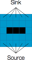
To solve for the large input, we need to look at the problem from a different point of view. It is known that the maximum flow problem is the dual of the minimum cut problem. That is, the maximum flow from the source to the sink is equal to the minimum capacity (or vertex capacity in our case) that needs to be removed (cut) from the graph so that no flow can pass from the source to the sink. It turns out that for this problem, it is easier to find the minimum cut than the maximum flow. That is, we need to determine the minimum number of cells (vertices) to be removed so that the source becomes disconnected from the sink.
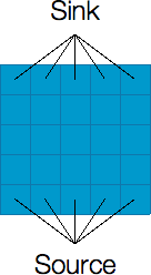
Let’s look at the example shown above. The left figure shows a river without any buildings. The source is connected to all cells at the bottom and the sink is connected to all cells at the top. The maximum flow from the source to the sink is 5. Looking at the structure of the river, It is obvious that to make a valid cut (via removing cells) that disconnects the source and the sink, the cut must form a path from the left side of the river to the right side of the river. The right figure shows the minimum cut solution where we remove the cells (highlighted with yellow color) to cut the river from left to right so that the source is now disconnected from the sink (i.e., no water can flow from the source to the sink anymore). Observe that the minimum cut (number of cells removed) is equal to the maximum flow.
Now, let’s look at examples where we actually have buildings. Since the cells covered by a building behave the same as removed cells (i.e. they do not allow water to flow through them), we can take advantage of the buildings to minimize the number of cells we need to remove to make a valid cut. See an example below where we have one building.
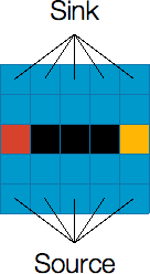
The left figure shows a river with an alien building in the middle. To disconnect the source from the sink, we only need to remove two more cells: one cell that connects the left side of the river to the left side of the building (highlighted with red color), and another cell that connects the right side of the building to the right side of the river (highlighted with yellow color). Thus, the minimum cut (and consequently the maximum flow) of this graph is 2.
Minimum cut as shortest path
With the above insights, we can rephrase our problem as follows: find the shortest path from the left side of the river to the right side of the river where the vertices are the buildings and the edge-cost between two buildings is the shortest distance between them. Note that the shortest distance between two buildings is the number of cells we need to remove to cut the region between the two buildings. If you are not familiar with shortest path algorithms, you can read up this tutorial. To see how the shortest path algorithm works to solve our problem, we show it for the example in the figure below.
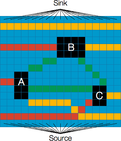
Remember that the black cells are buildings, and the other colored cells are water. The red cells show the shortest paths from the left side of the river to the three buildings while the yellow cells show the shortest paths from the right side of the river to the buildings (the top yellow edge connects the left side to the right side). The green cells show the distance from one building to the other, e.g. the distance between building A and B is 4.
To find a valid cut, we need to form a path from the left side of the river to the right side by going through the colored cells (other than blue and black cells). In the example above, the minimum cut is formed by the shortest path from the left side of the river to A (with distance 2) then from A to B (with distance 4) then from B to the right side of the river (with distance 5). Thus the minimum number of cells (minimum cut) that needs to be removed to disconnect the source and the sink is 11 cells, which is equal to the maximum flow.
To compute the distance between two buildings, it is enough to just look at their gap in the horizontal direction or vertical direction, and take the maximum of the two. The horizontal gap would be essentially the smallest distance between the two buildings if you were to project the two buildings on the horizontal (x) axis (likewise for the vertical gap). For example, building A and building B has 2 unit of vertical gap and 4 unit of horizontal gap. The distance from A to B is the one with the greater gap (i.e., 4 for the horizontal gap). Note that the vertical gap between building A and C is 0 as they overlap in their projection on the vertical (y) axis.
When computing the gap, we can imagine the left side and right side are buildings too (with infinite height). For those, we compute the horizontal gap only and ignore the vertical gap.
One may wonder about the case where there is another building between any two buildings. It means the actual distance between the two buildings can be shorter (by taking advantage of the building in between). This occurs when we look at the distance between building A and C. The actual gap between and A and C is 9 but due to the presence of building B, the distance is reduced to 8 (i.e. the sum of distance between A and B, and distance between B and C). Since we run a standard shortest path algorithm, it should take advantage of the buildings in between (i.e., the algorithm will not pick the edge (with higher distance) between A and C and instead go for the shorter distance through another building).
Analysis — D. Trie Sharding
We are given M distinct set of strings S. We want to assign these strings into N servers so that each server has at least one string. Each server then builds a trie from the strings it is assigned to. You are to find string assignments where the total number of nodes in the trie in all the servers is the maximum possible, also need to report the total number of different assignments.
To solve this problem, we first build a trie for the strings in S, then we compute the answers from that trie. To help with our explanation, we will use a different set of strings than the one provided in the problem statement. We use: AA, AB, AAA, B, with N = 3 servers. The corresponding prefixes for our example are “”, “A”, “AA”, “AAA”, “AB”, and “B”. The following figure shows the trie for these strings. Please refer to this tutorial if you are not yet familiar with tries.
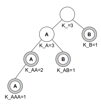
The nodes with double circles signify that its prefix is in the set of strings S. For each node p, the prefix of the node is defined as the string formed by concatenating the characters from the root to that node. The value K_p where p is the prefix of the node is explained in the following paragraph.
Before describing K_p, let’s discuss T_p. For a prefix p, let T_p be the number of strings that contain prefix p. In our example, the corresponding values for T_p are: T_=4, T_A=3, T_AA=2, T_AAA=1, T_AB=1 and T_B=1. Let us imagine an optimal assignment where the number of nodes is the maximum possible, we will describe how we compute an optimal assignment in a subsequent paragraph. In the optimal assignment, let us assume that a particular prefix p will appear the maximum number of times allowed (we will discuss this fact later). But the number of times the prefix can appear in an optimal assignment is capped by the number of servers N. In our example, the empty string can potentially appear a maximum of only 3 times instead of 4 (remember T_=4), the reason being that there are only 3 servers it can appear in! To account for this fact where T_p is capped by N, let us define another number K_p. For each prefix p let K_p be min(N, T_p). Therefore, K_p is the maximum number of times a prefix p can appear in any assignment. Going back to our problem, we note that maximizing the number of nodes is essentially equivalent to finding an assignment where each prefix p appears K_p times (if possible), and also to figure out the number of different assignments that have the maximum number of nodes.
Determine maximum number of nodes:
To generate an assignment with the maximum total number of nodes across all servers, we will use a greedy method. First, we sort the provided strings lexicographically. In our example, the provided strings are: AA, AB, AAA, B. Sorting it lexicographically will result in the sequence AA, AAA, AB, B. Let’s examine this sorted sequence. From our definition above, prefix p appears as a prefix for T_p strings. We claim that, after sorting the strings the prefix p will be in T_p consecutive strings in sorted order. Referring to our example, if we were to consider the prefix A, it appears in 3 strings which appear consecutively in the sorted sequence. Similarly AA appears as a prefix two times, and trivially the empty string appears four times.
We now describe a greedy strategy to assign the strings to servers. We will assign the sorted string #i to server #i mod N. In our example with three servers, we would have the following assignment: {AA,B}, {AAA}, and {AB}, i.e. the first and fourth strings get assigned to the first server, while the second and third strings get assigned to the second and third servers respectively. If instead we had two servers, we would have the assignment: {AA,AB}, {AAA,B}. We claim that this greedy assignment will give us the optimal assignment maximizing the number of nodes, resulting in each prefix p appearing K_p times on different server. The reason why each prefix p appears K_p times is because of an earlier argument where we pointed out that each prefix p appears in T_p consecutive strings. When assigning strings sequentially to the N servers, this will result in prefix p appearing in min(N, T_p) nodes, which is K_p. Therefore to compute the maximum number of nodes, it is sufficient to find the sum of K_p for all prefix p.
Count number of assignments with maximum number of nodes:
Before proceeding with the explanation, we would like to briefly talk about combinations. We can use Pascal’s triangle to precompute combinations. Each addition and multiplication operations are done modulo 1,000,000,007 (the modulo value is what our problem requires). For the purposes of this editorial, let’s say we precompute and save combinations in Choose(n, k) which chooses ‘k’ elements from ‘n’ elements. By definition, Choose(n, k) where n < k is defined to be zero.
Let us assume we already built the trie for strings S and for each node (with prefix p) in the trie, we already computed K_p (the maximum number of servers that this node with prefix p can be assigned to). We can traverse the trie using post-order traversal and compute the number of ways W_p to distribute the current node’s subtree among K_p servers, we will describe how we compute W_p in subsequent paragraphs. Note that the subtree of node p contains all the strings with prefix p. Since the root (node with prefix p = “”) is the prefix for all strings, we will have the final answer when we finish processing the root node.
Let’s examine the trivial case when we visit the leaf nodes during our traversal. A leaf node represents a whole string. Since we can only put one string in exactly one server, thus K_p = 1 for all leaf nodes p. Also, there is exactly one way to put a single node on a single server, thus W_p = 1 for all leaf nodes p.
Now, let’s examine the case of non-leaf (internal) nodes. After visiting all the children nodes c of node p, we can then compute W_p by using the following information:
- K_c: the number of servers assigned for each child node c.
- W_c: the number of assignments that yield the maximum number of nodes for each child node c.
- K_p: the number of servers assigned to this node p. Note that whenever a node is assigned to some server, all of its parent nodes also have to be assigned to the same server. Therefore, it is not possible to put any node on more servers than its parent node will be on, therefore K_p >= K_c.
- Whether prefix p is a whole string (i.e. it is one of the strings in set S).
To compute W_p for internal nodes p, we first need to compute:
- C1: the number of ways to choose which children go to which of the K_p servers
- C2: the number of ways to arrange the subtrees of each child c on its K_c servers
- C3: the number of ways to put the node's string (if prefix p is one of the strings in the set S, e.g. the node labeled K_AA in the figure above) to K_p servers
W_p is the product of C1, C2 and C3. C2 is the product of W_c of all the children c of node p because each child can assign its nodes to servers independently.
We can combine the computation for C1 and C3. If the prefix p is one of the strings in S (as in the node labeled K_AA in the figure above), then we can add an artificial leaf child node to node p. After adding an artificial leaf child node, computing C1 also covers computing C3. Note that the computation for C1 does not depend on the children's W_c. To compute C1, we only need the values of K_c. That is, to compute the number of ways to choose which children goes to which of the K_p servers, we only need to know the number of servers each child c is assigned to (i.e. the value K_c). To combine C3 into C1 computation, we can add a artificial child node c with K_c = 1.
We now proceed with the computation for C1. C1 can be computed via dynamic programming. We can store the values of K_c for all the child nodes in a list (including the case for C3, i.e. add K_c=1 for an artificial child) and we want to assign these child nodes into K_p servers such that for each child, no two children is assigned to the same server (since we want to maximize the number of servers used) and all K_p servers are used (i.e. none of the servers are empty). To better illustrate the computation, we explain it in terms of counting colored marbles.
Counting colored marbles:
At this point, we can think of the list of K_c as a collection of different colored marbles. Each entry in the list gives us the number of marbles of a particular color. The question is -- how many ways can we distribute these marbles into K bins (i.e. K_p servers) in such a way that each bin contains at least one marble and no bin contains two marbles of the same color? Notice that a bin translates to a server in our problem. Also, note that none of the servers can be empty therefore there should be at least one marble per bin.
The "at least one marble in each bin" condition is tricky, so we start by ignoring it and instead compute the number of distributions that have at most one marble of each color in each bin, but may have empty bins. This will lead to overcounting. Let us first focus on marbles of one color. If we have x marbles of some color, then they must go into x different bins (out of K bins). There are Choose(K, x) combinations to do such distributions. To generalize it to all colors, we multiply Choose(K, x) for each element x in the list. Let’s call this quantity OC_K to denote over counting for K. The quantity OC_K is over counting because when distributing the colored marbles to K servers, some of the servers might be empty. We in fact need to compute OC_i for all ‘i’ between 1 and K, you'll see why we need OC_i in a minute. Computing OC_i is similar to computing OC_K, but instead of K, we use i i.e. we multiply Choose(i, x) for each element x in the list.
We explain this idea of computing OC_i with a few examples. If the list contains {1, 2, 2, 3}, and the number of bins is 4, then OC_4 is Choose(4, 1) * Choose(4, 2) * Choose(4, 2) * Choose(4, 3). Note that if any of the values in the list is greater than number of bins i, then OC_i will be zero, e.g. if we have the same list but the number of bins is 2, then OC_2 is Choose(2, 1) * Choose(2, 2) * Choose(2, 2) * Choose(2, 3) but Choose(2, 3) is zero! Therefore OC_2 is also zero. Intuitively, the reason why it is zero is the following: We are counting the number of ways we can place 3 marbles in 2 bins such that each bin can have at most one marble, but that is impossible! Therefore it is zero.
So now, let’s focus on adding back the "no empty bins" condition. Now that we have OC_i for all values of ‘i’, we have the number of distributions into 'i' bins with some bins being potentially empty. How many distributions are there with no empty bins? Let's call this value Count_i. Note that Count_K is actually the answer we want. First off, we point out that Count_1 = OC_1. Why? The reason is because OC_1 is counting the number of ways we can place all the colored marbles into one server. This means there cannot be any empty servers because there is only one server to begin with! Hence Count_1 = OC_1.
To recap, we know OC_i and we also know Count_1 and we would like to compute Count_K. To do so, let’s look at the problem of computing Count_i. To do so, we will use OC_i. For a second, let us imagine how we would compute OC_i if we knew Count_i. It would be:
OC_i = sum(Count_a * Choose(i, i-a) for a in [1, i])Let us explain this formulation. Remember, OC_i is counting for distributions when some of the bins out of the ‘i’ bins are empty. Let us say there are ‘a’ non-empty bins therefore there are ‘i-a’ empty bins. There are Choose(i, i-a) ways to choose ‘i-a’ empty bins from ‘i’ bins. We will now fill the ‘a’ non-empty bins with marbles, which is actually given by Count_a!
We can switch the LHS and RHS of the above formulation, and rewrite the resulting LHS as follows:
Count_i * Choose(i,0) + sum(Count_a * Choose(i, i-a) for a in [1, i-1]) = OC_i
Note that Choose(i, 0) is 1. Therefore, after rearranging the above formulation, we get:
Count_i = OC_i - sum(Count_a * Choose(i, i-a) for a in [1, i-1])
This way, we can compute Count_i iteratively: first compute Count_2, then Count_3, and so on until we finally compute Count_K. Count_K is the number of ways to distribute the colored list of marbles into K bins in such a way that each bin contains at least one marble and no bin contains two marbles of the same color.
Please refer to rng..58’s implementation which implements the counting idea discussed above.