Google Code Jam Archive — Round 1A 2014 problems

This problem is looking for the minimum number of switches that need to be flipped so that all devices can be charged at the same time. All devices can be charged at the same time if each of the outlets can be paired with exactly one device and vice versa. An outlet can be paired with a device if both have the same electric flow after flipping some switches.

We observe that flipping the same switch two times (or an even number of times) is equivalent to not flipping the switch at all. Also, flipping the same switch an odd number of times is equivalent to flipping the switch exactly once. Thus, we only need to consider flipping the i-th switch once or not at all.

Let’s define a flip-string of 0s and 1s of length L as a way to flip the switches. If the i-th character of the string is 1, it means we flip the i-th switch (otherwise we do not flip the i-th switch). A flip-string is good if the resulting outlets’ electric flows (after the flips) allow all the devices to be charged at the same time. We can check whether a flip-string is good by flipping the bits in the outlets’ electric flow according to the flip-string and then checking whether each device’s electric flow can be matched exactly to one outlet with the same electric flow and vice versa. We can use hashing to perform the check and thus the complexity to check whether a flip-string is good is O(LN). Note that we can (optionally) encode the flip-string into a 64-bit number and reduce the complexity of the check to O(N).

Brute force algorithm:

A naive brute force solution is to try all the 2^L possible flip-strings and check whether it is a good flip-string and keep the one that has the least number of 1s in the string (i.e., it has the minimum number of flips). The time complexity of this algorithm is O(2^L * LN). For the small dataset where the maximum for L is 10, this brute force algorithm is sufficient. However, it is really slow for the large dataset where L can be as large as 40.

Better algorithm:

To improve the naive brute force algorithm we need two more observations. First is that there are only a few good flip-strings. If we can efficiently generate only the good flip-strings, we can improve the algorithm complexity significantly. The second observation is that given a device’s electric flow (of L bits) and an outlet’s electric flow (of L bits), we can generate a flip-string that will flip the outlet’s electric flow such that it matches the device’s electric flow. There are only N² possible pairs of devices and outlets. Thus, only N² flip-strings need to be generated. Note that the generated flip-strings may or may not be a good flip-string. However, all other flip-strings that are not generated by any pair is guaranteed to not be a good flip-string. With these observations, we can reduce the complexity of the naive algorithm down to O(N² * LN), which is fast enough for the large input.

The last (optional) observation we can make is that since a device must be plugged in to exactly one outlet, we can further reduce the number of possible flip-strings from N² down to N. The N possible flip-strings can be generated by pairing any one device with the N outlets.

Brute force algorithm:

Given a tree with N nodes, there are 2^N subsets of nodes that can be deleted from the tree. The brute force algorithm is to simply check all possible node deletions and pick the one where the remaining nodes form a full binary tree and the number of nodes deleted is minimum. Note that when a set of nodes are deleted from the tree, the remaining nodes may not be a tree anymore (since the tree may become disconnected).

Let’s say there are M remaining nodes after deletion. One way to check whether the remaining nodes form a full binary tree is to first check whether it is still a tree. This can be done by performing a simple breadth-first or depth-first search to check that the remaining nodes are in one connected component. Next, we need to find a root in that tree where all its subtrees have either zero or two children. This leads to an O(M²) algorithm for checking if the remaining nodes form a full binary tree.

Another way to check whether a graph is a full binary tree is via counting which is linear O(M):

• For the trivial case where M equals to 1, it is a full binary tree.
• For M > 1, it must satisfy that there is exactly one node having degree two and the rest of the nodes must have degree either one or three. Also, the number of remaining edges must be equal to M - 1 to signify that it is a tree, and not a disconnected graph.

Therefore, using different methods for checking whether the resulting graph is full binary tree or not you end up with a brute force algorithm that runs in O(2^N * N²) or O(2^N * N), which is sufficient to solve the small dataset. But it is not sufficient to solve the large dataset where N = 1000. In the following sections, we address the large dataset.

Quadratic algorithm:

The insight to the quadratic algorithm is that minimizing the number of deleted nodes is equivalent to maximizing the number of nodes that are not deleted.

Let’s pick a root for the tree. The parent-child relationship is defined based on the chosen root. For each node, we will make a decision to delete it or keep it with the goal of maximizing the size of the full binary subtree. We now investigate the various cases for each node. If a node has only one child, then we have to remove that child (as it violates the full binary tree condition of having 0 or 2 children). Therefore, the size of that subtree is only one node (i.e. we only count the node itself). If it has more than one candidate children, we have to pick two of them as the children of the node. But which two? We pick the two which retain the maximum number of nodes in their own subtrees, which we will demonstrate later.

We can implement the above idea via a greedy post-order depth-first-traversal from a chosen root. During the traversal, we determine the maximum number of nodes we can retain in each subtree to form a full binary tree. The function maxSubtreeNodes(node, parent) is as follows:

• The function’s parameters are the current node and its parent.
• If the current node has 0 or 1 children then the number of nodes in this subtree is 1.
• Otherwise, we have at least two subtrees and we should recursively call the function for each child of the current node. Remember, we want to maximize the number of nodes retained in the current node’s subtree, therefore we keep the two children that have the largest subtrees rooted at those children. We return the size of the two largest subtrees + 1 (1 to account the current node).

Finally, given this function the minimum number of nodes to be deleted for a given root node is:

N - maxSubtreeNodes(root, 0)  // 0 as the root does not have a parent.

We can run the maxSubtreeNodes(root, 0) function by picking each of the N nodes as the root. We pick the root node that minimizes N - maxSubtreeNodes(root, 0). As maxSubtreeNodes(root, 0) is a depth-first-traversal on a tree, it runs in O(N) time. Also, we run the traversal N times picking each node as the root. Therefore, the time complexity is O(N²).

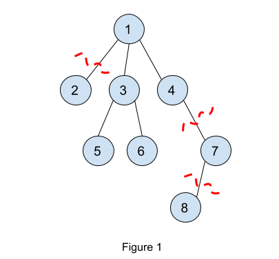
Figure 1 shows an example where we demonstrate running maxSubtreeNodes(1, 0). Node 8 is deleted as it is the only child for node 7. Then node 7 is deleted for the same reason. After that, node 1 will have to choose only two children among nodes 2, 3, and 4. These 3 subtrees have sizes 1, 3, and 1, respectively. So node 1 will choose the maximum two subtrees which are nodes 3 and 4 (note we could choose node 2 instead of node 4 too). So for maxSubtreeNodes(1, 0), the maximum number of nodes to keep is 5 (nodes 1, 3, 4, 5, and 6). Equivalently, the minimum number of nodes to be deleted is 3 (nodes 2, 7 and 8).

Here is the pseudo-code for this algorithm:

minDeletions = infinity
for root = 1 to N:
  minDeletions = min(minDeletions, N - maxSubtreeNodes(root, 0))

def maxSubtreeNodes(currentNode, parent):
  maximumTwoNumbers = {}  // Structure that keeps track of 
  // the maximum two numbers.
  for x in neighbors of currentNode:
     if x == parent:
       continue
     update maximumTwoNumbers with maxSubtreeNodes(x, currentNode)
  if size of maximumTwoNumbers == 2:
    return 1 + sum(maximumTwoNumbers)
  return 1

Linear algorithm:

The previous quadratic algorithm is sufficient to solve the large dataset but you might be interested in a solution with better time complexity. We present here a linear time algorithm which is based on the quadratic time algorithm.

In the quadratic algorithm, we take O(N) to compute the size of the largest two subtrees for any root node (remember, we brute force over all N possible root nodes). So our goal in the linear time algorithm is to compute the size of the largest two subtrees for any node in constant time. To do so, we will precompute the three largest children subtrees (not only two unlike in the quadratic algorithm). We will explain why we need three largest children in a subsequent paragraph.

So let's define our precomputation table structure. It is a one-dimensional array of objects called top3, which is defined as follows:

  class top3:
    class pair:
      int size
      int subtreeRoot
    pair children[3]  // children is sorted by the size value.
    int parent

In the greedy DFS function maxSubtreeNodes(node, parent), there are only 2 * (N-1) different parameter pairs for the function (a parameter pair is the node, parent pair, and also there are exactly N-1 edges in any tree). The key to our linear algorithm is to run DFS once on the given tree from some root node (say from node 1), and during this traversal for every node, to store the three largest subtrees among its children while also keeping track of the parent of the node. We will explain later why we need to keep track of the parent. This DFS traversal will be O(N) as it visits every node exactly once.

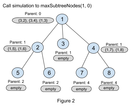
Figure 2 is an illustration figure for the stored top3 objects for every node after calling maxSubtreeNodes(1, 0). For node 2, {1, 5} means the subtree rooted at the child node 5 has maximum size 1, and “Parent: 1” means the parent of node 2 is 1.

But still after doing this precomputation there is something missing in our calculation. We assumed that node 1 is the root but in the original quadratic algorithm, we need to try all nodes as root. We now show how we can avoid having to try all nodes as root. In the function described above, for any node its parent is not considered as a candidate to be put in that node’s top3 children array. We now describe an example to show how we account for the parent of a particular node. In the example, we will use the parent’s information to update the top3 array for the current node.

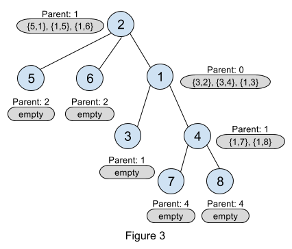
We describe a local update process to fix the top3 array for node 2. Remember that node 2’s parent is node 1 (see Figure 2). Let us pretend that node 2 is picked as the root (shown in Figure 3). We then look at its parent’s (node 1’s) top3 array. Note that the top element in the top3 array for node 1 is in fact node 2! We update node 2’s top3 array using node 1’s top3 array, therefore we exclude the result for node 2 from node 1’s top3 array. After excluding node 2 from the top3 array of node 1, the resulting pair describing node 1 is {5, 1} (i.e. size of subtree rooted at node 1 excluding node 2 is 5: nodes 1, 3, 4, 7 and 8). We now update the top3 array for node 2 with {5,1}. Therefore, now node 2’s top3 array is: {5,1}, {1,5}, {1,6}, and the size of the largest full binary tree rooted at node 2 is 7 (5 + 1 from the first two children, and 1 to count node 2 itself).

We perform the local update process described in the previous paragraph in a pre-order depth-first-traversal starting from node 1. Note that when doing the local update, excluding the current node from its parent’s top3 array might result in an array with only one element. In such cases, the parent’s subtree (excluding the current node) should be of size 1.

Well, you might be still wondering why we need the three largest subtrees and not two. Observe in Figure 3, if we had stored only the top 2 instead of the top 3 subtrees in node 1 (meaning only {3,2} and {3,4}) and we excluded node 2 during the local update, then we will only have the pair {3,4} which describes node 4 but ignores node 3! This would be incorrect as node 3 is part of a full binary tree rooted at node 1. Therefore we keep information for the largest three subtrees.

This problem is a bit unusual for a programming contest problem since it does not require the solution to be exactly correct. In fact, even the best solutions may get wrong answer due to random chance. That being said, there exist solutions that can correctly classify, with high probability of success, whether a permutation was generated using the BAD algorithm or the GOOD algorithm. One such solution is to generate many samples of BAD and GOOD permutations and to look at their frequency distribution according to some scoring functions. Knowing the distributions of the scores, we can create a simple classifier to distinguish the GOOD and the BAD permutations. Note that while the solution seems to be very simple, the amount of analysis needed and the number of trial and errors to produce a good scoring function are not trivial. The rest of the analysis explains the intuition to construct a good scoring function.

What makes a GOOD permutation?

If a permutation of a sequence of N numbers is GOOD, then the probability of each number ending up in a certain position in the permutation is exactly 1 / N. In the GOOD algorithm, this is true for every step. In the first step, the probability of each number ending up in the first position is exactly 1 / N since the length of the sequence is initially N. Now the number in the first position is fixed (i.e., it will not be swapped again in the next steps), we can ignore it in the second step and only consider the remaining sequence of N - 1 numbers. Whichever number that gets chosen in the second step did not get chosen in the first step ((N - 1) / N chance), and got chosen in the second step (1 / (N - 1) chance), so every number has a 1 / N chance of ending in the second position. Continuing this logic, in the end, every number has a uniform 1 / N probability to end up in any position in the permutation sequence.

Why is the BAD algorithm BAD?

Let’s examine the BAD algorithm. At first, the BAD algorithm may look “innocent” that in step i it picks an element at random position and swaps it to the element at position i. However, a deeper look will reveal that the direction in which i is progressing makes the resulting permutation become BAD (i.e., it is not uniform). To see this, imagine we are currently at step i and we pick a random number X at position j where j happens to be less than i. Then X can never be swapped to lesser position than i in the next steps. The number X can only be swapped to higher positions in the permutation. This creates some bias in the permutation.

Let’s examine the frequency of seeing the number i that ends up in position j in the permutation for all i,j. We illustrate the frequency in the figures below. The x-axis (from left-to-right) is the original position of the numbers (from 0 to N - 1). The y-axis (from bottom-to-top) is the position of numbers in the permutation generated by the algorithm (from 0 to N - 1). For this illustration, we use N = 100. We run each algorithm (the GOOD and the BAD separately) 20K times and record the event that number i (in the original position) ends up in position j (in the permutation). The intensity of the pixel at position x=i, y=j represent the frequency of the events. The darker the color represent the higher frequency of occurrence.

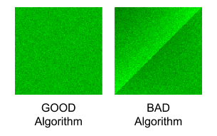
We can observe that the GOOD algorithm uniformly distributes the numbers from the original positions to the resulting permutation positions. While the BAD algorithm tends to distribute the lower numbers in the original positions to the higher positions in the permutation (notice the darker region on the top left corner).

A Simple Classifier

With the above insights, we can devise a simple scoring function to classify the BAD permutation by counting the number of elements in the permutation that move to lower positions compared to its original position. See the following pseudo-code for such a scoring function:

def f(S):
  score = 0
  for i in 0 .. N-1:
    if S[i] <= i:
      score++
  return score

The scoring function f takes in a permutation sequence S of length N and returns how many numbers in the permutation sequence that ends up at position that is less than or equal to its original position. If the permutation sequence S is generated by the GOOD algorithm, we expect that the score should be close to 500 for N = 1000. If S is generated by the BAD algorithm, we expect that the score should be significantly lower than 500 (since the lower numbered elements tends to move to higher position). If we run 10K samples for each algorithm and plot the frequency distribution of the scores, we will get the following graph:

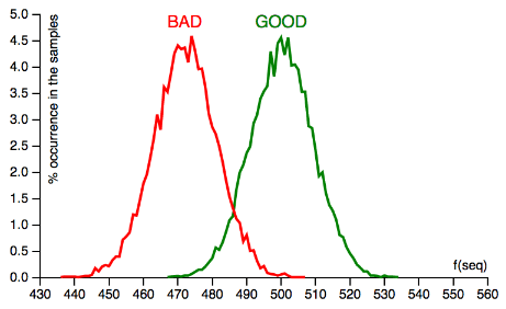
The GOOD algorithm produces samples with scores clustered near 500 while the BAD algorithm produces samples with scores near 472. Knowing these scores, we can build a very simple classifier that decides whether a given permutation sequence S is generated by the GOOD or the BAD algorithm with high probability. We can simply check the score of f(S) whether it is near 472 (BAD) or 500 (GOOD), as depicted in the following pseudo-code:

if f(S) < (472 + 500) / 2:
  S is produced by the BAD algorithm
else:
  S is produced by the GOOD algorithm

How accurate is the classifier?

The good thing about being a programmer is that we do not always need formal proofs. We can roughly guess the accuracy of the classifier by generating a number of GOOD / BAD permutations each with 50% probability and check how many permutations are correctly classified using our simple classifier. According to our simulation, the simple classifier achieves around 94.05% accuracy. The simple classifier is good enough to correctly solve 109 test cases out of 120 test cases: this will happen in roughly 94.58% of all inputs. In the unlucky situation that your input is in the other 5.42%, you can download another one. 5.42% seems to be a lot to be given to chance though. What if you were only allowed one submission? In the next section we'll explore one idea out of many that offer higher chances of success.

Naive Bayes Classifier

P(GOOD | S) = P(S | GOOD) * P(GOOD) / (P(S | GOOD) * P(GOOD) + P(S | BAD) * P(BAD))

where:

• P(S | GOOD) is the probability that S is generated by the GOOD algorithm
• P(S | BAD) is the probability that S is generated by the BAD algorithm
• P(GOOD) is the probability that the permutation is chosen from the GOOD set
• P(BAD) is the probability that the permutation is chosen from the BAD set

Since we know that P(GOOD) and P(BAD) is equally likely since each algorithm has the same probability to be used, then we can simplify the rule to:

P(GOOD | S) = P(S | GOOD) / (P(S | GOOD) + P(S | BAD))

If P(GOOD | S) > 0.5, it means that the permutation S is more likely generated by the GOOD algorithm. By substituting P(GOOD | S) with the right hand side of the rule in P(GOOD | S) > 0.5 and performing some algebraic manipulation, we can further simplify the expression to P(S | GOOD) > P(S | BAD).

We know the exact value for P(S | GOOD) is 1/N! since there are N! possible permutations. Hence, we only need to find P(S | BAD). If we can find P(S | BAD), we will have an optimal algorithm. Unfortunately, we do not know how to efficiently compute P(S | BAD) precisely. The best algorithm we know is intractable for large N = 1000.

Nevertheless, we can borrow an idea from machine learning and make a simplifying Naive Bayes assumption: let’s assume that the movement of each element is independent. Now we can approximate P(S | BAD):

P(S | BAD)  ≈  P(S[0] | BAD) * P(S[1] | BAD) * ... * P(S[N-1] | BAD)

where P(S[0] | BAD) is the probability that the first element in a random permutation generated by BAD is in fact S[0]. Without the independence assumption, we would have terms like P(S[1] | BAD + S[0]), which means "the probability that the second element is in fact S[1] given that BAD is used to generate the permutation and that the first element is S[0]". Naive Bayes allows us to remove the italicized assumption, which makes the calculation tractable (but not completely accurate).

To be fair, we should make the same simplifying assumption for P(S | GOOD). Luckily, this is easy; in the GOOD algorithm, each element has a 1 / N chance of moving to each position, so P(S | GOOD) = 1 / N^N regardless of what S we are given.

Now, let’s see how we can implement the Naive Bayes classifier. Let P_k[i][j] be the probability that number i ends up at position j after k steps of the BAD algorithm. We are interested in the probabilities where k = N (i.e., after N steps have been performed). We can compute P_k from P_k-1 in O(N²) time by simulating all possible swaps. P₀ is easy; nothing has moved, so we just have the identity matrix. See the pseudo-code below. P_k[i][j] is the prev[i][j] variable which will contain the probability of number i ends up at position j after k steps generated by the BAD algorithm.

  prev[i][i] = 1.0 for all i, otherwise 0.0  // An identity matrix.
  pmove = 1.0 / N  // Probability of a number being swapped.
  pstay = 1.0 - pmove  // Probability of a number not being swapped.

  for k in 0 .. N-1:
      for i in 0 .. N-1:
          next[i][k] = 0
          for j in 0 .. N-1:
              next[i][k] += prev[i][j] * pmove  // (1)
              if j != k:
                  next[i][j] = prev[i][j] * pstay +
                               prev[i][k] * pmove  // (2)
      Copy next to prev

Note for (1): P[i][k] for the next step is equal to: (P[i][j] in the previous step) * (move probability to k). Note for (2): P[i][j] for the next step is equal to: (P[i][j] in the previous step) * (staying probability at j) + (P[i][k] in the previous step) * (move probability to j).

The above algorithm runs in O(N³). It may take several seconds (or minutes if implemented in a slow scripting language) to finish. However, we can run this offline (before we download the input), and store the resulting probability matrix in a file. Note that the above algorithm can also be optimized to O(N²) if needed. See Gennady Korotkevich's solution for GCJ 2014 Round 1A for an implementation.

Next, we compute the approximation probability of P(S | BAD) as described previously.

  bad_prob = 1.0
  for i in 0 .. N:
    bad_prob = bad_prob * prev[S[i]][i]

Finally, to produce the output, we compare it with P(S | GOOD) and see which one is greater.

  good_prob = 1.0 / N^N
  if good_prob > bad_prob:                             
    S is produced by the GOOD algorithm
  else:
    S is produced by the BAD algorithm

Note that the pseudo code above is dealing with very small probability that may cause underflow in the actual implementation. One way to avoid this problem is to use sum of the logarithm of the probabilities instead of the product of the probabilities.

Empirically, the Naive Bayes classifier has a success rate of about 96.2%, which translates into solving at least 109 cases correctly out of 120 in 99.8% of all inputs.

Finally, in this editorial we described two methods to solve this problem. There are likely other solutions that perform even better and we invite the reader to try come up with such solutions.