Google Code Jam Archive — Round 2 2010 problems
Overview
Round 2 of the 2010 Google Code Jam was quite challenging - a big step up from some of the Round 1 problems!
Problem A was not too hard conceptually, but the unusual diamond shape required our contestants to design their own way of implementation, and this proved to be difficult. Problem B was a dynamic programming puzzle about the upcoming FIFA world cup that required viewing it in the right way to make progress... Fortunately, our contestants were very good at this! Problem C is a wonderful mathematical puzzle with a simple depth first search solution. Our last problem has deep roots in computational geometry, and it required tremendous implementation skill to get everything right during a timed contest. A big congratulations is due to halyavin and bsod for their correct solutions!
The top three contestants were bmerry, ZhukovDmitry, and winger, who all solved 3 and a half problems in around 2 hours. Congratulations to them, as well to all of the 500 advancers to Round 3. There is only one more round to go until the on-site finals in Dublin!
Cast
Problem A. Elegant Diamond Written and prepared by Bartholomew Furrow and Igor Naverniouk.
Problem B. World Cup 2010 Written by Xiaomin Chen. Prepared by Ante Derek.
Problem C. Bacteria Written by Cosmin Negruseri. Prepared by Cosmin Negruseri and John Dethridge.
Problem D. Grazing Google Goats Written by Cosmin Negruseri. Prepared by John Dethridge and David Arthur.
Contest analysis presented by David Arthur, Xiaomin Chen, Petr Mitrichev, and Cosmin Negruseri
Solutions and other problem preparation provided by Derek Kisman and Petr Mitrichev.
A. Elegant Diamond
Problem
The king has hired you to make him an elegant diamond. An elegant diamond is a two-dimensional object made out of digits that's symmetric about a horizontal and a vertical axis. For example, the following four shapes are elegant diamonds:
   2       8      3     7
  3 3     8 8    2 2
 4 1 4     8      3
  3 3
   2
These three shapes are diamonds, but are not elegant:
  2       1        3
 1 1     1 2      1 1
  1     1 1 1    3 1 3
         2 1      1 1
          1        2
These three shapes are not diamonds:
  1     2     8   8
 1 1   222      0
        2     00000
The king will start by giving you a diamond, which may not be elegant. Your job is to make it elegant by enhancing it, adding digits on to make a bigger diamond. Because you don't want to spend too much money, you want to do it with as little cost as possible.
Definitions
A diamond of size k is 2k-1 lines of digits, 0-9, separated by single spaces, organized in the following way:
- Line i (1 ≤ i ≤ k) contains k-i spaces, then i digits separated by single spaces.
- Line i (k < i < 2k) contains i-k spaces, then 2k-i digits separated by single spaces.
An elegant diamond of size k is a diamond of size k with the following two symmetry properties:
- Horizontal symmetry: Let ci be the number of digits on line i. The jth digit on line i (where j=1 for the first digit) must be the same as the ci+1-jth digit.
- Vertical symmetry: The jth digit on line i (where i=1 for the first line) must be the same as the jth digit on line 2k-i.
A diamond of size k can be enhanced by adding digits to it. The result of enhancing a diamond of size k has the following properties:
- The result is a diamond of size ≥ k.
- The original diamond is part of the result. In other words, there exist some X and some Y such that, for all values of i and j such that the jth character of the ith line of the original is a digit (as opposed to a space), the j+Xth character on the i+Yth line of the result is also a digit and it's the same as the jth character on the ith line of the original.
The cost of enhancing a diamond is equal to the number of digits in the result of the enhancement, minus the number of digits in the original diamond.
Input
The first line of the input gives the number of test cases, T. T test cases follow. Each test case consists of a single integer k in a line on its own, followed by a diamond of size k.
Output
For each test case, output one line containing "Case #x: y", where x is the case number (starting from 1) and y is the minimum cost required to enhance the given diamond into an elegant diamond. If the diamond is already elegant, y=0.
Limits
Memory limit: 1GB.
1 ≤ T ≤ 100.
Small dataset (Test set 1 - Visible)
Time limit: 30 seconds.
1 ≤ k ≤ 10.
Large dataset (Test set 2 - Hidden)
Time limit: 60 seconds.
1 ≤ k ≤ 51.
Sample
4
1
0
2
 1
2 2
 1
2
 1
1 2
 1
3
  1
 6 3
9 5 5
 6 3
  1
Case #1: 0
Case #2: 0
Case #3: 5
Case #4: 7
Explanation
There are four cases. The first two cases start as elegant diamonds of size 1 and 2, respectively, and don't need to be enhanced; so the cost is 0. The third case can be enhanced to look like:
  3
 1 1
1 2 1
 1 1
  3
There are several possible enhancements, but this is one with the lowest possible cost, which is 5. In the fourth case we can enhance the diamond into the following elegant diamond:
   9
  1 1
 6 3 6
9 5 5 9
 6 3 6
  1 1
   9
...for a cost of 7.
B. World Cup 2010
Problem
After four years, it is the World Cup time again and Varva is on his way to South Africa, just in time to catch the second stage of the tournament.
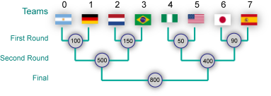
In the second stage (also called the knockout stage), each match always has a winner; the winning team proceeds to the next round while the losing team is eliminated from the tournament. There are 2P teams competing in this stage, identified with integers from 0 to 2P - 1. The knockout stage consists of P rounds. In each round, each remaining team plays exactly one match. The exact pairs and the order of matches are determined by successively choosing two remaining teams with lowest identifiers and pairing them in a match. After all matches in one round are finished, the next round starts.
In order to help him decide which matches to see, Varva has compiled a list of constraints based on how much he likes a particular team. Specifically, for each team i he is willing to miss at most M[i] matches the team plays in the tournament.
Varva needs to buy a set of tickets that will guarantee that his preferences are satisfied, regardless of how the matches turn out. Other than that, he just wants to spend as little money as possible. Your goal is to find the minimal amount of money he needs to spend on the tickets.
Tickets for the matches need to be purchased in advance (before the tournament starts) and the ticket price for each match is known. Note that, in the small input, ticket prices for all matches will be equal, while in the large input, they may be different.
Example
A sample tournament schedule along with the ticket prices is given in the figure above. Suppose that the constraints are given by the array M = {1, 2, 3, 2, 1, 0, 1, 3}, the optimal strategy is as follows: Since we can't miss any games of team 5, we'll need to spend 50, 400, and 800 to buy tickets to all the matches team 5 may play in. Now, the constrains for the other teams are also satisfied by these tickets, except for team 0. The best option to fix this is to buy the ticket for team 0's first round match, spending another 100, bringing the total to 1350.
Input
The first line of the input gives the number of test cases, T. T test cases follow. Each case starts with a line containing a single integer P. The next line contains 2P integers -- the constraints M[0], ..., M[2P-1].
The following block of P lines contains the ticket prices for all matches: the first line of the block contains 2P-1 integers -- ticket prices for first round matches, the second line of the block contains 2P-2 integers -- ticket prices for second round matches, etc. The last of the P lines contains a single integer -- ticket price for the final match of the World Cup. The prices are listed in the order the matches are played.
Output
For each test case, output one line containing "Case #x: y", where x is the case number (starting from 1) and y is the minimal amount of money Varva needs to spend on tickets as described above.
Limits
Time limit: 30 seconds per test set.
Memory limit: 1GB.
1 ≤ T ≤ 50
1 ≤ P ≤ 10
Each element of M is an integer between 0 and P, inclusive.
Small dataset (Test set 1 - Visible)
All the prices are equal to 1.
Large dataset (Test set 2 - Hidden)
All the prices are integers between 0 and 100000, inclusive.
Sample
2
2
1 1 0 1
1 1
1
3
1 2 3 2 1 0 1 3
100 150 50 90
500 400
800
Case #1: 2
Case #2: 1350
C. Bacteria
Problem
A number of bacteria lie on an infinite grid of cells, each bacterium in its own cell.
Each second, the following transformations occur (all simultaneously):
- If a bacterium has no neighbor to its north and no neighbor to its west, then it will die.
- If a cell has no bacterium in it, but there are bacteria in the neighboring cells to the north and to the west, then a new bacterium will be born in that cell.
Upon examining the grid, you note that there are a positive, finite number of bacteria in one or more rectangular regions of cells.
Determine how many seconds will pass before all the bacteria die.
Here is an example of a grid that starts with 6 cells containing bacteria, and takes 6 seconds for all the bacteria to die. '1's represent cells with bacteria, and '0's represent cells without bacteria.
000010
011100
010000
010000
000000

000000
001110
011000
010000
000000

000000
000110
001100
011000
000000

000000
000010
000110
001100
000000

000000
000000
000010
000110
000000

000000
000000
000000
000010
000000

000000
000000
000000
000000
000000
Input
The input consists of:
- One line containing C, the number of test cases.
- One line containing R, the number of rectangles of cells that initially contain bacteria.
- R lines containing four space-separated integers X1 Y1 X2 Y2. This indicates that all the cells with X coordinate between X1 and X2, inclusive, and Y coordinate between Y1 and Y2, inclusive, contain bacteria.
North is in the direction of decreasing Y coordinate.
West is in the direction of decreasing X coordinate.
Output
For each test case, output one line containing "Case #N: T", where N is the case number (starting from 1), and T is the number of seconds until the bacteria all die.
Limits
Time limit: 30 seconds per test set.
Memory limit: 1GB.
1 ≤ C ≤ 100.
Small dataset (Test set 1 - Visible)
1 ≤ R ≤ 10
1 ≤ X1 ≤ X2 ≤ 100
1 ≤ Y1 ≤ Y2 ≤ 100
Large dataset (Test set 2 - Hidden)
1 ≤ R ≤ 1000
1 ≤ X1 ≤ X2 ≤ 1000000
1 ≤ Y1 ≤ Y2 ≤ 1000000
The number of cells initially containing bacteria will be at most 1000000.
Sample
1
3
5 1 5 1
2 2 4 2
2 3 2 4
Case #1: 6
D. Grazing Google Goats
Problem
Farmer John has recently acquired a nice herd of N goats for his field. Each goat i will be tied to a pole at some position Pi using a rope of length Li. This means that the goat will be able to travel anywhere in the field that is within distance Li of the point Pi, but nowhere else. (The field is large and flat, so you can think of it as an infinite two-dimensional plane.)
Farmer John already has the pole positions picked out from his last herd of goats, but he has to choose the rope lengths. There are two factors that make this decision tricky:
- The goats all need to be able to reach a single water bucket. Farmer John has not yet decided where to place this bucket. He has reduced the choice to a set of positions {Q1, Q2, ..., QM}, but he is not sure which one to use.
- The goats are ill-tempered, and when they get together, they sometimes get in noisy fights. For everyone's peace of mind, Farmer John wants to minimize the area A that can be reached by all the goats.
Unfortunately, Farmer John is not very good at geometry, and he needs your help for this part!
For each bucket position Qj, you should choose rope lengths so as to minimize the area Aj that can be reached by every goat when the bucket is located at position Qj. You should then calculate each of these areas Aj.
Example
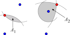
In the picture below, there are four blue points, corresponding to the pole positions: P1, P2, P3, and P4. There are also two red points, corresponding to the potential bucket positions: Q1 and Q2. You need to calculate A1 and A2, the areas of the two shaded regions.
Input
The first line of the input gives the number of test cases, T. T test cases follow. Each test case begins with a line containing the integers N and M.
The next N lines contain the positions P1, P2, ..., PN, one per line. This is followed by M lines, containing the positions Q1, Q2, ..., QM, one per line.
Each of these N + M lines contains the corresponding position's x and y coordinates, separated by a single space.
Output
For each test case, output one line containing "Case #x: A1 A2 ... AM", where x is the case number (starting from 1), and A1 A2 ... AM are the values defined above. Answers with a relative or absolute error of at most 10-6 will be considered correct.
Limits
Memory limit: 1GB.
All coordinates are integers between -10,000 and 10,000.
The positions P1, P2, ..., PN, Q1, Q2, ..., QM are all distinct and no three are collinear.
Small dataset (Test set 1 - Visible)
Time limit: 30 seconds.
1 ≤ T ≤ 100.
N = 2.
1 ≤ M ≤ 10.
Large dataset (Test set 2 - Hidden)
Time limit: 120 seconds.
1 ≤ T ≤ 10.
2 ≤ N ≤ 5,000.
1 ≤ M ≤ 1,000.
Sample
3
2 3
0 20
20 0
-20 10
40 20
0 19
4 2
0 0
100 100
300 0
380 90
400 100
1000 5
3 1
0 0
10 10
20 0
10 5
Case #1: 1264.9865911 1713.2741229 0.2939440
Case #2: 1518.9063729 1193932.9692206
Case #3: 0.0
Analysis — A. Elegant Diamond
On this very difficult round, even the first problem was pretty challenging. The constraints were fairly small, but it might not be clear how to even get started. After all, there are a lot of ways you can enhance a diamond!
Let's start off with a slightly simpler question: given a position (cx, cy), is it possible to enhance (i.e, extend) the given diamond into an elegant diamond centered at (cx, cy)? (Note that this center might be either at a number, or at a space between numbers, depending on whether the elegant diamond has even or odd side length.) The resulting diamond
would have to be symmetrical about the lines x = cx and y = cy. Specifically, this means that for each (x, y), the values in positions (x, y), (2cx - x, y), (x, 2cy - y), and (2cx - x, 2cy - y) all have to be equal. If the starting diamond already has two different values in one of these quartets, there's nothing we can do to change that.
Otherwise, it turns out that the diamond always can be extended to an elegant diamond with center at (cx, cy). For each of the quartets above where we have one value, we have to fill out the remaining values to be equal. After that, we can just enclose everything in a diamond shape and fill all remaining squares with 0. Here's an example:
  1
 2 3
5 6*6
 2 3
  1
Let's try to extend this to an elegant diamond centered at the *. First, we fill in all quartets, and then we extend to a proper diamond by adding 0's:
                             0
  1           1 1           1 1
 2 3         2 3 2         2 3 2
5 6*6  -->  5 6*6 5  -->  5 6*6 5
 2 3         2 3 2         2 3 2
  1           1 1           1 1
                             0
Done!
This is pretty clearly the smallest extension with the given center, so all we need to do is try each possible center, and choose the one that gives the smallest possible elegant diamond.
Of course, there are a lot of possible centers, but there is no need to consider one completely outside of the bounding box of the original diamond. We can always move such a center onto the edge of the bounding box without creating any inconsistencies, and that will lead to a smaller diamond in the end.
So in summary: we need to iterate over all possible centers contained within the original diamond, check if there is an elegant extension with that center, and then take the smallest of these. As always, please take a look at some of the correct submissions to see some full implementations!
By the way, the solution presented here is O(n^4), which is fast enough for this problem. Faster solutions do exist though, and you might enjoy looking for them.
Analysis — B. World Cup 2010
Reformulation
In the analysis, we will turn the picture upside-down. This conforms to the usual convention that the root of a binary tree is drawn on top. This is actually easy to do implementation-wise. We just read the input numbers in reverse order; the element at position 0 is the root, i.e., the final match, and for any node i, its two children are indexed at 2i+1 and 2i+2. In our particular solution, we include nodes for the teams as well as for the matches, so our graph is a rooted complete binary tree, where all the internal nodes are matches, and all the leaves are the teams.
Perhaps it is clear that the solution will be dynamic programming on the tree. There are many ways to do it, but some can be much more complicated than others. Let us introduce one solution that is very simple. It is based on the following reformulation of our problem.
Let us color a node yellow if we are going to buy the ticket for the corresponding match. For each leaf (a team), the path to it from the root has P internal nodes. We call a plan good if no matter what the outcomes of the matches are, we will never miss more than M[i] matches for team i. We have
(*) A plan is good if and only if for every teamThis is indeed a conceptual leap in solving the problem. For in the new form, we no longer need to worry about the outcome of any particular match. And once it is stated, it is very easy to justify. We leave the justification to the readers.i, the path from the root to the leaf corresponding to team i has at leastP-M[i]yellow nodes.
Simple solutions for small inputs and large inputs both follow easily from this reformulation.
Small dataset
For the small dataset the best plan must be upwards closed, i.e., if a node is yellow, all the nodes on the path from the root to it must all be yellow. One can prove this by using (*) and noting that all the prices are the same, and you can always get a cheaper plan if you push some yellow node upwards.
So, one solution for the small dataset looks like this: For each team i, we find the path from root to it, and color the topmost P-M[i] nodes yellow. It can be done in linear time by a simple modification of depth first search.
The justification and the implementation details are a nice piece of dessert. We leave them to the readers.
Large dataset
We use dynamic programming on the tree. Let us just define the subproblems clearly. For any node a and any number b between 0 and P, let P(a, b) be the problem
If there areAnd we can use a impossibly big answer to indicate that the condition can not be satisfied.byellow nodes on the path from the root toa(not includinga), what is the cheapest way to color the nodes in the sub-tree rooted at a, such that all the leaves in this sub-tree satisfy the condition in (*)?
Once the DP is set up, the code follows easily. For each internal node there are just two choices, color it yellow or not. We provide an excerpt from one of the judges' solutions:
i64 A[1<<11][11];  // answers for the dynamic programming.
i64 inp[1<<11];    // input, in reversed order.
int P;

// rooted at a, already buy b tickets from above.
i64 dp(int a, int b) {
  i64& r=A[a][b];
  if(r>=0) return r;
  if(a>=((1<<P)-1)) {r=(b>=(P-inp[a]))?0:1LL<<40; return r;}
  r=std::min(
      inp[a]+dp(2*a+1,b+1)+dp(2*a+2,b+1),
      dp(2*a+1,b)+dp(2*a+2,b));
  return r;
}

int main() {
  int T;
  cin>>T;
  for (int cs=1; cs<=T; ++cs) {
    cin>>P; int M=(2<<P)-1;
    for (int i=0; i<M; i++) cin>>inp[M-1-i];
    memset(A, -1, sizeof(A));
    cout << "Case #" << cs << ": " << dp(0, 0) <<endl;
  }
  return 0;
}
Analysis — C. Bacteria
The fact that the input is a set of rectangles is not essential to this problem. We just wanted to limit the amount of data you had to download to test your program. So let us forget about the rectangles, and instead consider any initial configuration of n bacteria on the grid. The challenge here is to compute the answer fast. A turn by turn simulation will not be good enough. We are going to aim for an O(n) solution instead.
Examples
One way to start attacking this problem is to look at examples. The Bacteria game is pretty fun to play around with after all! Here are some examples you can try:
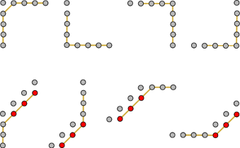
- A rectangle of
HbyWbacteria. - A
HbyWrectangle where the bacteria only lie on the four boundary edges. - Bacteria along a "type 1" diagonal (a southwest/northeast diagonal).
- Bacteria along a "type 2" diagonal (a northwest/southeast diagonal).
- A random path where each pair of bacteria are connected either horizontally, vertically, or along a type 1 diagonal.
X + Y = C, the right-most point containing a bacterium X = Xmax, and the bottom-most point containing a bacterium Y = Ymax. We claim that after one turn, the configuration will still be a single connected piece, the highest diagonal will become X + Y = C+1, and the max X and Y coordinates will not change. This will continue until the final second when we come down to a single point (Xmax, Ymax). So the number of turns before everything disappears is Xmax + Ymax - C + 1.
One thing we note is that the 3rd and 4th examples behave very differently. In the 3rd example, the number of bacteria decreases by 1 in each turn, while in the 4th, all the bacteria disappear immediately.
Solution
Define a graph on the bacteria. Two bacteria are neighbors if they are adjacent on the grid via a horizontal line, a vertical line, or a type 1 diagonal. We begin by finding the connected components of this graph.
This may seem like a simple definition, but it is really the key to solving the whole problem. It is quite similar to the more common graph where each grid node has 8 neighbors, one in each compass direction, except we do not consider the 2 directions along a type 2 diagonal. Remember the 3rd and 4th examples above? If we start with n nodes, there is just one connected component in the former, but n connected components in the latter.
We observe that after each turn, a connected component will give birth to a new connected component (unless it was a single point and disappears), and different components will not become connected together. See the details in the next section.
So, the answer is the maximum elimination time over all the components. For a single piece (i.e., connected component), we find the highest type 1 diagonal X + Y = C, as well as the maximum coordinates Xmax and Ymax. The number of turns for that piece to disappear is then Xmax + Ymax - C + 1.
Justification
Our solution depends very heavily on several key observations. If you try some examples, you should be able to convince yourself empirically that these observations just have to be true. But in the interest of completeness, we will also sketch out a more formal proof here.
In the following discussion, we will fix a configuration called the old state, and we will consider the new state obtained after one turn. When we talk about a connected piece, we will always assume the non-trivial case where there are at least 2 points in the piece.
For each bacterium in the new state, let us consider the reason why it is there. If it was in the old state, we credit the reason for its existence to the set of itself and its north and/or west neighbor. If it was not in the old state, we credit the reason for its existence only to the set of its north and west neighbors. In both cases, we call such a set the credit set for that single bacterium.
Proposition 1. If the old state is a single piece, and the highest type 1 diagonal is X + Y = C, then in the new state, the highest type 1 diagonal will become X + Y = C+1.
Proof. Consider a bacterium at position (X, Y) on the top diagonal of the old state. Since this is the top diagonal, that bacterium does not have a north neighbor or a west neighbor, and it will die. In particular, the diagonal X + Y = C will be completely empty in the new state.
Now pick the south-most bacterium in the old state on the diagonal X + Y = C. Let its position be (X, C-X). If there is also a bacterium at position (X+1, C-X-1) in the old state, there will be a bacterium at (X+1, C-X) in the new state (no matter whether it was in the old state or not). Otherwise, since (X, C-X) is part of a connected piece and it's on the highest diagonal, there will be a bacterium at either (X, C-X+1) or (X+1, C-X) in the old state, and by our rules, this bacterium will survive to the new state. Hence, in any case, we find at least one bacterium will be on the diagonal X + Y = C+1 in the new state, which proves the proposition.
The following two Propositions can be justified in the same way:
Proposition 2. If the old state is a single piece, the maximum X coordinate and the maximum Y coordinate will be unchanged in the new state.
To see Proposition 3, note that if the old state is connected, then any two credit sets can be joined by some path consisting of horizontal, vertical, and type 1 diagonal segments. As the following picture shows, any possible segment from such a path will give birth to connected segments in the new state:
Finally, we are going to prove that different pieces will not be merged together in a turn.
Proposition 4. If two bacteria are neighbors in the new state, then their credit set are all from the same piece in the old state.
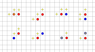
This is obviously true if both bacteria are also in the old state. Otherwise, it is one of the cases in the following picture. The two bacteria are the circled points. A blue point indicates that the bacterium was also in the old state, a red point indicates that the bacterium was only in the new state. Then the yellow stars represents the points in the credit sets. In any situation we either reach an impossible configuration, or get to a point where it is clear the credit sets are connected.
Analysis — D. Grazing Google Goats
This problem is tough from both the implementation side and the algorithm side. In the analysis, we will begin by explaining some general concepts that show how the task is actually very similar to convex hull. We will then go into the particulars needed to build a solution and to prove that it is right. The resulting code isn't as scary as the length of the analysis makes you think.
Let us just focus on one bucket Q at a time. The problem asks us to choose rope lengths: i.e., for each pole position, we need to choose the radius of the circle centered at that pole. The common area will be the intersection of all these circles. It is clear that decreasing the radius of any circle will not increase the intersection. Therefore, we want the lengths to be as small as possible. Obviously, for each pole Pi, PiQ is the smallest length we can pick so that the goat can still reach the bucket. Our main task is to efficiently compute the common intersection area of these circles.
From the limits of this problem, it is also clear that computing the intersection in Ω(N2) will be too slow. We are aiming for an algorithm that will, for each bucket, compute the intersection in time O(N log N).
The intersection is a convex shape where the boundary consists of arcs of the circles. One can prove in various ways (some of the reason will be obvious below) that each circle will only contribute at most one such arc. We will mostly focus on how to compute these arcs -- to which circle does it belong, where does it stop and where does it start. Once all this is computed, it is relatively easy to get the area.
Some theoretical background
While this section is not absolutely necessary for solving the problem, it will provide some nice insights. Once we have seen the problem from a few different angles, the solution will be conceptually clear and very natural.
So, first of all, note that all the circles we consider pass through a common point Q. If you have not seen it before, it is now our honor to introduce to you the beautiful geometric transformation called inversion. It takes Q as the center. And each point X ≠ Q is mapped to a point X' where QX and QX' are in the same direction, and the lengths satisfy |QX| |QX'| = 1.
Here is one very nice property of inversion: Every circle passing through the center point Q is mapped to a line that does not pass Q, and vice versa. And the interior of the circle is mapped to a half-plane that does not include Q. For our problem, the intersection of the N circles is then mapped to the intersection of N half-planes. For more details on inversion, we refer you to the Wikipedia page on inversive geometry.
We leave it to the reader to verify that, if the intersection is not empty, then we can rotate the plane such that Q is above all the half-planes. And the intersection of the half-planes is bounded by something called the lower envelope of line arrangements. The segments of the lower envelope are exactly the images of the arcs in the circle intersection from our original problem.
Then there is a concept of duality in computational geometry that maps each line y = ax + b to the point (a, -b). The lower envelope is mapped by this transformation to the upper convex hull of the set of corresponding points.
So, our problem is indeed equivalent to the convex hull problem and the lower envelope of line arrangements problem. Both subjects are well studied and there are simple O(N log N) algorithms for both.
Out of these three settings, perhaps the algorithm for line arrangement is the simplest to visualize: Sort the lines by their slopes, and add them one by one. In each step, the existing lower envelope will be cut by the new line in two parts. The time for sorting is O(N log N), and the amortized complexity for the rest is O(N).
Solution to our problem
The previous section suggests a couple approaches that begin with explicitly doing an inversion about Q. In this section, we will discuss a direct solution to the problem, where we do not need to view the problem using the transformations from the previous section. Note that it will be in some ways equivalent to the above algorithm we introduced for line arrangements.
Let's look from Q along a straight ray. The intersection of this ray with each circle will be either just Q, or a segment between Q and the second intersection point of this ray with the boundary of the circle. That means that in order to build the area required in the problem statement, we need to find the circle "closest" to Q in each direction from it. Let's denote each direction by its polar angle, which is defined up to a multiple of 2π.
We start by considering just one circle. Suppose the polar angle of a ray that goes from Q towards the center of that circle is φ. When the polar angle of a ray goes from φ-π/2 towards φ, the distance from Q to the second intersection point with that ray increases from 0 to the diameter of the circle. When the polar angle continues from φ towards φ+π/2, the distance decreases back to 0. When the polar angle changes from φ+π/2 to φ+3π/2 (the latter is the same as φ-π/2, where we started), the intersection of the ray with the circle is just Q.
Now consider two circles, one with center at polar angle φ (remember, all polar angles discussed here are relative to Q) , another one with center at polar angle ξ, and suppose 0 < φ - ξ < π. Then we'll see the following as we turn the ray originating from Q: starting from polar angle ξ-π/2 until φ-π/2 the ray will intersect only the second circle; from φ-π/2 the ray will intersect both circles, but the intersection point with the first circle will be closer to Q until the circles intersect; after the intersection and until ξ+π/2 the ray will still intersect both circles but the second is now closer; and from ξ+π/2 until φ+π/2 the ray will only intersect the first circle.
The important thing about the two circles case discussed above is that in the range of polar angles where the ray intersects both circles (and that's exactly the range we care about in finding the intersection area). The situation is very simple: before the intersection point one circle is closer to Q, after the intersection point another circle is closer to Q.
Now suppose we have many circles. First, we find the polar angle of the center of each circle, and thus also find the range of polar angles where a ray going from Q intersects each of the circles. We can then intersect all those ranges of polar angles to obtain a small range [α, β] of polar angles where the ray would intersect all circles. If this range is empty, then we already know there's no intersection.
Now let's start adding circles one by one, starting from the one with the smallest polar angle. You might ask, what does "smallest" mean when we're on a circle? Luckily, here we have less than full circle: since all circles intersect all rays in [α, β] range, the polar angles of all centers are between β-π/2 and α+π/2. That leaves us a segment of length less than π where we have a definite order.
As we're adding the circles, we'll maintain which circle is closest for each angle from [α, β]. For example, after adding the first circle it will be the closest for the entire [α, β] range. Now we add the second circle. Let's say the polar angle of the intersection point between two circles is γ. If you look carefully at the above analysis, you'll find that:
- When γ is less than α, the first circle is still the closest for the entire [α, β] .
- When γ is between α and β, the second circle is the closest for [α, γ], and the first circle is the closest for [γ, β].
- When γ is more than β, the second circle is now closest for the entire [α, β] .
Here we rely on the fact that we process circles in increasing order of the polar angle of their center.
Now look at the general case. Suppose before adding circle number i we have the following picture: on [α, γ1] circle j1 is the closest; on [γ1, γ2] circle j2 is the closest; ...; on [γk-1, β] circle jk is the closest.
Consider the polar angle δ of the intersection point between circle i and circle j1. There are 3 ways it could compare with the range where j1 is the closest:
- When δ is less than α, it means that circle
j1is closer than circleion the entire [α β] segment, and we can just stop processing circleisince it doesn't affect the answer. - When δ is between α and γ1, we now have that circle
iis the closest on [α, δ], and circlej1is the closest on [δ, γ1]. After doing this change, we can also stop processing circleisince circlej1will be closer to the center all the remaining way. - Finally, when δ is more than γ1, we can forget about circle
j1since circleiis closer than it on the entire [α, γ1] segment. In that case we continue processing circleiby comparing it with circlej2, and so on.
That's it! After we do this processing for all circles, we know the contour of the intersection figure, and we continue by computing its area.
The above algorithm requires a data structure that maintains a list of arcs with integer tags, allowing us to change the first arc, remove the first arc, and add a new first arc. The simplest way to get this data structure is to just use a stack where the first ac would be on the top, and the last one would be on the bottom.
The running time for the above algorithm can be estimated using amortized analysis as follows. When processing each circle, we do at most two "push to stack" operations, and one or more "pop from stack" operations. That means the total number of push operations is O(N), and since the number of pop operations can't be greater than the number of push operations (there'd be nothing to pop!), it's also O(N), giving us the total runtime of O(N). However, we must also remember the step where we sort all circles by the polar angle of their center, so overall runtime is O(N log N).
We've so far avoided discussing the low-level computational geometry needed for this problem. In the above solution we required two geometric routines: find the polar angle of the other intersection point of two circles which have the first intersection point at origin; and find the area of a figure that is bounded by arcs.
The first routine is straightforward if you can already intersect circles (a useful thing to know how to do!); alternatively, you could derive the formulas for the polar angle directly. The second one is slightly more tricky: first, we split the figure into "rounded triangles" with rays going from Q and having polar angles γ1, γ2, ..., γk-1. Each rounded triangle has two straight sides (one of those might have zero length) and one circular side. We can then split the rounded triangle into the corresponding triangle plus the round part (a sliced off part of a circle). You have probably seen how to compute the area of a triangle before - one good approach is the "shoelace formula". To calculate the rounded area, it helps to start with a "pie slice" from the center, whose area is a simple fraction of the total circle area, and then add or subtract triangle areas.
Of course there is a lot to do here, but that's why we made it Problem #4!